REVIEW 3 major objections 3 minor 29 references
Hierarchical Bayesian Operational Modal Analysis: Theory and Computations
T0 review · 3 major / 3 minor · reviewed 2026-08-14 · deepseek-v4-flash
Pith's one-line read This paper claims that a hierarchical Bayesian model separates per-record identification precision from record-to-record variability in modal identification.
desk verdict A genuinely new embedding of Au's fast Bayesian FFT likelihood into a Gaussian hierarchy, with careful calculus, but the Gaussian hyperprior puts real posterior mass on negative damping and Remark 5's unit-norm claim is simply wrong. read the letter →
The pith
A machine-rendered reading of the paper's core claim, the machinery that carries it, and where it could break.
The reading
What carries the argument
The load-bearing object is the Gaussian hyperprior of Eq. (13), an unknown-mean, unknown-covariance distribution over the dynamical parameters, namely modal frequency, damping ratio, and mode-shape components. It works because each data set's stage-one likelihood is approximated by a Gaussian, making the integral over each data set's parameters conjugate; the closed-form marginal in Eq. (20) is what turns the whole framework into a tractable two-level model. The same conjugacy produces the gain-matrix update for each data set's refined posterior in Eqs. (23)-(24) and the MAP/ensemble identities in Eqs. (38)-(39). For small numbers of data sets, an eigenbasis reparameterization of the hypercovariance fixes the unidentifiability of off-diagonal correlations by estimating only eigenvalues, with eigenvectors frozen at the approximate MAP estimate.
What would settle it
Simulate a known linear system with a prescribed frequency spread across records; estimate the same data with the paper's Laplace-based hierarchy and with a full MCMC that does not Laplace-approximate each likelihood. If the posterior predictive intervals for a new record differ beyond Monte Carlo error, the stage-one Gaussian is carrying the conclusion.
Extended reading notes
Core claim
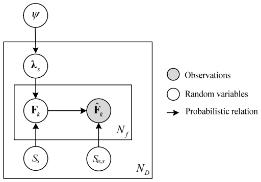
The central claim is that the ensemble variability of modal parameters across independent vibration data sets is itself a Bayesian quantity. After the paper replaces each data set's likelihood with its Laplace approximation, $N(\hat{\lambda}_s,\hat{\Sigma}_{ss})$, the data-set-specific dynamical parameters are conditionally independent draws from a Gaussian hyperdistribution with unknown mean $\mu_\lambda$ and covariance $\Sigma_{\lambda\lambda}$. Integrating out the per-data-set parameters in closed form gives the marginal posterior of the hyperparameters in Eq. (20), and MAP estimation of that posterior yields the ensemble mean of the per-data-set estimates, with a covariance that shrinks the ensemble sample covariance by the average within-data-set covariance in Eqs. (38)-(39). The paper thus interprets what frequentist practice treats as sample moments as Bayesian hyperparameters, while retaining the per-record posteriors for identification precision.
Load-bearing premise
The framework's tractability rests on each data set's likelihood being faithfully represented by the Laplace Gaussian $N(\hat{\lambda}_s,\hat{\Sigma}_{ss})$ with $\hat{\Sigma}_{ss}$ treated as known in the second-level update; short records, weakly excited modes, or structured prediction errors break that approximation, and the second level cannot repair first-level bias.
Editorial extensions
If this is right
- Fusing many short ambient records yields one posterior that includes test-to-test scatter, so reported modal uncertainties need not be artificially small.
- When the number of data sets is large, the dual Laplace algorithm gives closed-form MAP hyperparameters with analytical gradients, avoiding expensive sampling.
- Each data set's posterior is corrected toward the ensemble through a gain matrix; the covariance for that experiment shrinks when other data sets agree with it.
- The posterior predictive distribution for an unobserved operating condition gives a direct uncertainty bound on modal parameters for future records, not just for the measured ones.
Reading between the lines
- The paper's MAP/ensemble identities suggest a general principle beyond modal analysis: for any inverse problem with repeated independent experiments, a Gaussian hyperprior converts empirical ensemble moments into Bayesian estimates with a variance correction for per-experiment precision.
- A practical diagnostic the paper does not develop: the hypercovariance's eigenvalues can be monitored across data-set batches; sudden growth would signal a changing operating condition or damage, while stable small eigenvalues indicate purely identificatory scatter.
- If the Laplace stage is replaced by a non-Gaussian but cheap surrogate, such as a skew or heavy-tailed approximation, the same two-level conjugacy is lost; whether a variational approximation preserves the separation of precision and variability is a testable open extension.
Signed reviews
Editorial analysis
A structured set of objections, weighed in public.
Referee Report
Summary. The paper develops a hierarchical Bayesian framework for operational modal analysis from multiple vibration data sets. Each data set's posterior is first approximated by a Laplace/Gaussian approximation of the fast Bayesian FFT likelihood (Eq. (12)); a Gaussian hyperprior is then placed on the modal parameters (Eq. (13)), and marginalization yields a closed-form hyperparameter posterior (Eq. (20)). The authors propose an MCMC sampler (Algorithm 1) and a dual Laplace approximation (Algorithm 2), derive MAP estimates whose initial values recover the ensemble mean and covariance (Eqs. (38)-(39)), and add an eigenbasis simplification for the hyper covariance matrix (Algorithm 3). Two experimental examples, a three-story shaking-table structure and a cable footbridge, are used to demonstrate that the framework captures both identification precision and between-dataset variability.
Significance. If the model-support issue raised below is resolved, the paper would be a useful contribution: it extends hierarchical Bayesian ideas to frequency-domain Bayesian OMA, provides explicit Gaussian-marginalization and gradient/Hessian derivations (Appendices A and C), and offers two practical computational routes. The algebraic core is standard and internally consistent, and the examples are plausible demonstrations on real structural data. The claimed connection between hierarchical MAP estimates and frequentist ensemble statistics is conceptually interesting, even though the 'proof' is conditional on simplifying assumptions. The main weakness is that the Gaussian hyperprior and its posterior predictive assign significant probability to physically inadmissible modal parameters, which undermines the central claim of a coherent posterior over physical modal parameters.
major comments (3)
- [§3.1 Eq. (13); §3.2.3 Eq. (41); Remark 5] The Gaussian hyperprior in Eq. (13) has unrestricted support over the reparameterized dynamical parameters lambda = [f, xi, phi^T]^T, and the posterior predictive in Eq. (41) inherits that support. The first-level model in Section 2 constrains damping ratios to be positive and mode-shape vectors to unit Euclidean norm (Remark 2), so the hierarchy is not, as claimed, a coherent posterior over physical modal parameters. This is not a hypothetical concern: Table 1 (sampling method) reports xi_1 mean 0.039 and SD 0.0883, giving P(xi_1 < 0) = Phi(-0.039/0.0883) approximately 0.33; Table 3, mode 2, reports xi_2 mean 0.006 and SD 0.0793, giving P(xi_2 < 0) approximately 0.47. Remark 5's assertion that unit-norm constraints are automatically preserved is also incorrect: the mean of a Gaussian over mode-shape components is not generally on the unit sphere, and even a degenerate Gaussian with zero radial variance has support on a tangent hyperplane, not on the sphere. The authors should either restrict the hyperprior to the physically valid support (e.g., truncated Gaussian or a reparameterization with xi>0 and phi on the sphere) or explicitly reframe the posterior as one over unconstrained working parameters and discuss the consequences for the physical interpretation.
- [§4.3 and Algorithm 3] The eigenbasis simplification fixes the eigenvectors of the hyper covariance matrix to those of the initial estimate obtained from Eq. (39). This is not merely a computational acceleration; it changes the target distribution by imposing an ad hoc constraint on the hyper covariance that is absent from the hierarchical model in Section 3. If the initial estimate of the eigenvectors is poor, the resulting posterior and posterior predictive will be biased in a way not accounted for by the reported uncertainties. The identifiability issue is real, but Algorithm 3 should be presented explicitly as an approximation that alters the model, and the authors should discuss when it is safe (e.g., when the likelihood surface is flat in those directions) or should validate it with simulations.
- [§3.1 Eq. (12); §4.2.2] The framework treats the first-level Laplace covariance matrices Sigma_hat_s as known when constructing the second-level update in Eq. (17). For short records, weakly excited modes, or high prediction error, the stage-one Gaussian approximation in Eq. (12) can be biased, and the second level cannot repair that bias. The paper states that each data set is 'sufficiently large' and gives a diagnostic via the Hessian inverse in Table 2, but this is only used for one example. The claim that the framework effectively separates identification precision from ensemble variability should be qualified by explicit regime conditions, and a sensitivity check (e.g., varying record length or number of data sets) would substantially strengthen the scope claims.
minor comments (3)
- [Abstract and §4.2.1] The abstract says the MAP/ensemble coincidence is 'proved', but Eqs. (38)-(39) are derived under the assumption of equal first-level covariance matrices for all data sets. Please state this assumption in the theorem or abstract, and clarify that under heterogeneous precisions the MAP estimate is a precision-weighted mean (Eq. (37)), not the unweighted ensemble mean.
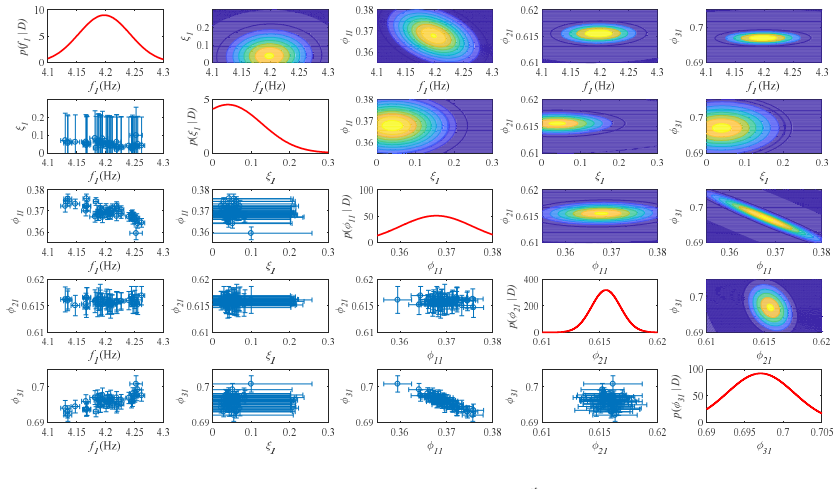
- [Section 5] The examples compare the hierarchical posterior predictive with the data-set-specific likelihoods from the same data sets used for inference. This demonstrates in-sample fit but does not validate the predictive distribution for new operating conditions. A leave-one-out or test-set evaluation would be more convincing evidence for the claimed capability to predict variability at unobserved conditions.
- [References and typesetting] Reference [61] duplicates reference [56], and references [69] and [72] appear to be the same manual; the reference list should be cleaned. In the provided text, several displayed equations (e.g., Eq. (13) and Eq. (27)) have garbled or ambiguous sub/superscripts; please ensure all notation is typeset unambiguously.
Circularity Check
Derivation is self-contained; no fitted input is renamed as a prediction.
full rationale
The central derivation chain is not circular. The marginal posterior of the hyperparameters in Eq. (20) is obtained by analytically integrating the product of two Gaussian densities (the Laplace-approximated likelihood and the Gaussian hyperprior), with the proof given in Appendix A via standard Gaussian identities. The MAP/ensemble-covariance relations in Eqs. (38)-(39) are derived by setting the gradient of the negative log marginal posterior, Eqs. (35)-(36), to zero under the stated equal-covariance assumption, and they are presented as initial estimates and as a conceptual variance decomposition rather than as an independently fitted quantity later renamed a prediction. The posterior predictive distribution in Eq. (41) is a plug-in Gaussian using the MAP hyperparameters, which is a standard Bayesian predictive calculation; its covariance is an estimator of between-dataset variability derived from the first-level MPVs, not a quantity that was fitted and then reported as a prediction by construction. Self-citations to Sedehi et al. are contextual and do not carry a load-bearing uniqueness claim or ansatz. The mathematically questionable assertion in Remark 5 that unit-norm constraints are automatically preserved is a correctness concern, not a circularity concern. No equation was found that reduces to its own input by construction.
Assumptions & free parameters
free parameters (4)
- hyper mean vector mu_lambda =
Table 1 (shaking table): f1 ~ 4.197-4.205 Hz, xi1 ~ 0.039-0.050; Table 3 (footbridge): f1 ~ 3.848 Hz
- hyper covariance matrix eigenvalues =
Standard deviations in Table 2, e.g., sigma_f ~ 0.0001, sigma_xi ~ 0.004-0.006
- per-dataset noise and modal force PSDs (S_i, S_ei) =
Not tabulated
- eigenvalue prior bound in U(0,0.1) =
0.1
assumptions (6)
- domain assumption Prediction errors in the FFT domain are i.i.d. complex Gaussian with constant PSD (Eq. 5)
- domain assumption Each dataset is long enough that the Laplace asymptotic approximation in Eq. (11) accurately represents the posterior and likelihood as Gaussian
- domain assumption Dynamical parameters across datasets are exchangeable draws from a multivariate Gaussian hyperdistribution (Eq. 13)
- domain assumption Datasets are statistically independent (Eqs. 14 and 16)
- ad hoc to paper Hyper covariance eigenvectors can be fixed to the eigenbasis of the initial sample estimate in Algorithm 3
- domain assumption Uniform priors for hyper mean and covariance parameters (Section 5.1, Eq. 44)
Cite this review
Pith. "Pith review of Hierarchical Bayesian Operational Modal Analysis: Theory and Computations." pith.science (2026). https://pith.science/paper/7725IGL4
@misc{pith2026190806370,
  author       = {Pith},
  title        = {Pith review of: Hierarchical Bayesian Operational Modal Analysis: Theory and Computations},
  year         = {2026},
  howpublished = {\url{https://pith.science/paper/7725IGL4}},
  note         = {Machine review of arXiv:1908.06370}
}
read the original abstract
This paper presents a hierarchical Bayesian modeling framework for the uncertainty quantification in modal identification of linear dynamical systems using multiple vibration data sets. This novel framework integrates the state-of-the-art Bayesian formulations into a hierarchical setting aiming to capture both the identification precision and the ensemble variability prompted due to modeling errors. Such cutting-edge developments have been absent from the modal identification literature, sustained as a long-standing problem at the research spotlight. Central to this framework is a Gaussian hyper probability model, whose mean and covariance matrix are unknown encapsulating the uncertainty of the modal parameters. Detailed computation of this hierarchical model is addressed under two major algorithms using Markov chain Monte Carlo (MCMC) sampling and Laplace asymptotic approximation methods. Since for a small number of data sets the hyper covariance matrix is often unidentifiable, a practical remedy is suggested through the eigenbasis transformation of the covariance matrix, which effectively reduces the number of unknown hyper-parameters. It is also proved that under some conditions the maximum a posteriori (MAP) estimation of the hyper mean and covariance coincide with the ensemble mean and covariance computed using the MAP estimations corresponding to multiple data sets. This interesting finding addresses relevant concerns related to the outcome of the mainstream Bayesian methods in capturing the stochastic variability from dissimilar data sets. Finally, the dynamical response of a prototype structure tested on a shaking table subjected to Gaussian white noise base excitation and the ambient vibration measurement of a cable footbridge are employed to demonstrate the proposed framework.
Figures

Figures from the paper (5 more)


Reference graph
Works this paper leans on
-
[4]
doi:10.1016/j.compstruc.2012.12.015. [22] S. - K. Au, Operational Modal Analysis - Modeling, Bayesian Inference, Uncertainty Laws, Springer, Singapore, 2017. doi:10.1007/978 - 981 - 10 - 4118 - 1. [23] S.K. Au, J.M.W. Brownjohn, J.E. Mottershead, Quantifying and ma naging uncertainty in operational modal analysis, Mech. Syst. Signal Process. 102 (2018) 13...
-
[12]
doi:10.1016/j.ymssp.2015.04.023. [38] H. - F. Lam, J. - H. Yang, J.L. Beck, Bayesian operational modal analysis and assessment of a full - scale coupled structural system using the Bayes - Mode - ID method, Eng. Struct. 186 (2019) 183 –
- [15]
-
[22]
doi:10.1111/j.2517 - 6161.1977.tb01600.x. [8] P. Verboven, P. Guillaume, B. Cauberghe, S. Vanlanduit, E. Parloo, Modal parameter estimation from input – output Fourier data using frequency - domain maximum li kelihood identification, J. Sound Vib. 276 (2004) 957 –
arXiv 2004
-
[29]
doi:10.1016/j.ymssp.2018.09.041. [62] V. Madar, Direct formulation to Cholesky decomposition of a general nonsingular correlation matri x, Stat. Probab. Lett. 103 (2015) 142 –
-
[95]
doi:10.1007/s13349 - 011 - 0009 - 5. [4] E. Reynders, R. Pintelon, G. De Roeck, Uncertainty bounds on modal parameters obtained from stochastic subspace identification, Mech. Syst. Signal Process. 22 (2008) 948 – 969. doi:10.1016/j.ymssp.2007.10.009. [5] E. Reynders, System identification methods for (operational) modal analysis: review and comparison, Ar...
-
[110]
doi:10.1016/j.jsv.2016.03.022. [49] I. Behmanesh, S. Yousefianmoghadam, A. Nozari, B. Moaveni, A. Stavridis, Uncertainty quantification and propagation in dynamic m odels using ambient vibration measurements, application to a 10 - story building, Mech. Syst. Signal Process. 107 (2018) 502 – 514. doi:10.1016/j.ymssp.2018.01.033. [50] M. Song, B. Moaveni, C...
-
[113]
doi:10.2514/1.I010264. [53] J.B. Nagel, B. Sudret, A unified framework for multilevel uncertainty quantification in Bayesian inverse problems, P robabilistic Eng. Mech. 43 (2016) 68 – 84. doi:10.1016/j.probengmech.2015.09.007. [54] O. Sedehi, L.S. Katafygiotis, C. Papadimitriou, A Time - Domain Hierarchical Bayesian Approach for model updating, in: 16th E...
Show all 29 references
-
[124]
doi:10.1007 /s11831 - 012 - 9069 - x. [6] H.E. Rauch, C.T. Striebel, F. Tung, Maximum likelihood estimates of linear dynamic systems, 49 AIAA J. 3 (1965) 1445 –
1965
-
[147]
doi:10.1016/j.spl.2015.03.014. [63] Z. Li, C.C. Chang, Adaptive quantification of noise variance using subspace technique, J. Eng. Mech. 139 (2013) 469 –
2013 doi
-
[155]
[35] W.J
doi:10.1016/j.ymssp.2014.07.027. [35] W.J. Yan, L.S. Katafygiotis, A nove l Bayesian approach for structural model updating utilizing statistical modal information from multiple setups, Struct. Saf. 52 (2015) 260 – 271. doi:10.1016/j.strusafe.2014.06.004. [36] W. - J. Yan, L.S...
2015 doi
-
[171]
doi:10.1016/j.ymssp.2014.08.016. [34] W. Yan, L.S. Katafygiotis, A two - stage fast Bayesian spectral density approach for ambient modal analysis. Part I: Posterior most probable value and uncertainty, Mech. Syst. Signal Process. 54 – 55 (2015) 139 –
2015 doi
-
[202]
52 [39] J
doi:10.1016/j.engstruct.2019.02.016. 52 [39] J. - H. Yang, H. - F. Lam, J.L. Beck, Bayes - Mode - ID: A Bayesian modal - component - sampling method for operational modal analysis, Eng. Struct. 189 (2019) 222 – 240 . doi:10.1016/j.engstruct.2019.03.047. [40] B. Li, A. Der Kiur...
2019
-
[220]
doi:10.1016/j.ymssp.2015.05.031. [29] Y. - C. Zhu, S. - K. Au , Bayesian operational modal analysis with asynchronous data, part I: Most probable value, Mech. Syst. Signal Process. 98 (2018) 652 – 666. doi:10.1016/j.ymssp.2017.05.027. [30] Y. - C. Ni, F. - L. Zhang, Fast Bayes...
2018 doi
-
[226]
doi:10.1061/(ASCE)EM.1943 - 7889.0000213. [21] S. Au, F. Zhang, Y. Ni, Bayesian operational modal analysis: Theory, computation, practice, Comput. Struct. 126 (2013) 3 – 1
2013
-
[231]
50 [17] L.S
doi:10.1016/S0266 - 8920(01)00004 - 2. 50 [17] L.S. Katafygiotis, K. - V. Yuen, Bay esian spectral density approach for modal updating using ambient data, Earthq. Eng. Struct. Dyn. 30 (2001) 1103 – 1123. [18] K. - V. Yuen, L.S. Katafygiotis, Bayesian Modal Updating using Compl...
2001 doi
-
[235]
doi:10.1016/j.compstruc.2018.08.018. [31] Y. - C. Zhu, S. - K. Au, J.M.W. Brownjohn, Bayesian operational modal analysis with buried modes, Mech. Syst. Signal Process. 121 (2019) 246 –
2019 doi
-
[263]
[32] F.L
doi:10.1016/j .ymssp.2018.11.022. [32] F.L. Zhang, H.B. Xiong, W.X. Shi, X. Ou, Structural health monitoring of Shanghai Tower during different stages using a Bayesian approach, Struct. Control Heal. Monit. 23 (2016) 1366 –
2016 doi
-
[416]
[27] F.L
doi:10.1002/stc.1679. [27] F.L. Zhang, Y.C. Ni, H.F. Lam, Bayesian structural model updating using ambient vi bration data collected by multiple setups, Struct. Control Heal. Monit. 24 (2017) 1 – 18. doi:10.1002/stc.2023. [28] F. - L. Zhang, Y. - C. Ni, S. - K. Au, H. - F. Lam...
2017 doi
-
[461]
doi:10.1061/ (ASCE)0733 - 9399(1998)124:4(455). [16] K. - V. Yuen, L.S. Katafygiotis, Bayesian time – domain approach for modal updating using ambient data, Probabilistic Eng. Mech. 16 (2001) 219 –
1998
-
[478]
doi:10.1061/(ASCE)EM.1943 - 7889.0000499. [64] Z. Feng, St ructural health monitoring using wireless sensor networks and Bayesian probabilistic methods, The Hong Kong University of Science and Technology, 2013. doi:10.14711/thesis - b1251919. [65] J. Ching, Y. - C. Chen, Trans...
2007
-
[533]
doi:10.1016/j.ymssp.2018.08.047. [37] S. - K. Au, Insights on the Bayesian spectral density m ethod for operational modal analysis, Mech. Syst. Signal Process. 66 – 67 (2016) 1 –
2016 doi
-
[688]
doi:10.1016/j.ymssp.2019.06.007. [61] O. Sedehi, C. Papadimitriou, L.S. Katafygiotis, Probabilistic hierarchical B ayesian framework for time - domain model updating and robust predictions, Mech. Syst. Signal Process. 123 (2019) 648 –
2019 doi
-
[815]
doi:10.1061/(ASCE)EM.1943 - 7889.0000385. [26] F. - L. Zhang, S. - K. Au, H. - F. Lam, Assessing uncertainty in operational modal analysis incorporating multiple setups using a Bayesian approach, Struct. Control Heal. Monit. 22 (2015) 395 –
2015
-
[847]
[13] E.T
doi:https://doi.org/10.1002/stc.424. [13] E.T. Jaynes, Information theory and statistical mechanics, Phys. Rev. 106 (1957) 620. [14] J.L. Beck, Statistical System Identification of Structures, in: 5th Int. Conf. Struct. Saf. R eliab., ASCE, San Francisco, California, 1989. ced...
1957 doi
-
[979]
doi:10.1016/j.jsv.2003.08.044. [9] J.R. Fonseca, M.I. Friswell, J.E. Mottershead, A.W. Lees, Uncertainty identification by the maximum likelihood method, J. Sound Vib. 288 (2005) 587 – 599. doi:10.10 16/j.jsv.2005.07.006. [10] T.J. Matarazzo, S.N. Pakzad, Sensitivity metrics f...
2005 doi
-
[1384]
doi:10.1002/stc.1840. [33] W. Yan, L.S. Ka tafygiotis, A two - stage fast Bayesian spectral density approach for ambient modal analysis. Part II: Mode shape assembly and case studies, Mech. Syst. Signal Process. 54 – 55 (2015) 156 –
2015 doi
-
[1450]
doi:10.2514/3.3166. [7] A.P. Dempster, N.M. Laird, D.B. Rubin, Maximum Likelihood from incomplete data via the E M algorithm, J. R. Stat. Soc. Ser. B. 39 (1977) 1 –
1977 doi
-
[1997]
doi:10.1061/(ASCE)0733 - 9399(1997)123:12(1219)
1219 – 1229. doi:10.1061/(ASCE)0733 - 9399(1997)123:12(1219). [59] C.E. Rasmussen, C.K.I. Williams, Gaussian processes for machine learning., 2004. doi:10.1142/S0129065704001899. [60] O. Sedehi, C. Papadimitriou, D. Teymouri, L.S. Katafygiotis, Sequentia l Bayesian estimation ...
1997 doi
Reviewed August 14, 2026 · model on record in the stance chip above.
Discussion (0). Continue with ORCID to comment.