Local Information Operators for Spatial Identifiability in Distributed-Parameter Inverse Problems in Computational Mechanics
Pith reviewed 2026-06-29 09:25 UTC · model grok-4.3
The pith
A linearized information operator on parameter perturbations quantifies spatial identifiability in distributed inverse problems.
A machine-rendered reading of the paper's core claim, the machinery that carries it, and where it could break.
Core claim
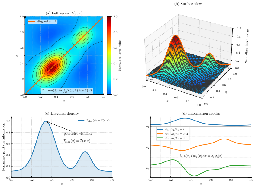
Around a nominal parameter field, the parameter-to-observation map is linearized and the likelihood contribution to posterior precision is interpreted as an operator on parameter-field perturbations. For locally linearized Gaussian models with parameter-independent covariance, this operator is equivalently Fisher information, Gauss-Newton data-misfit curvature, and a noise-weighted sensitivity Gramian. The framework separates pointwise visibility from spatial identifiability. The diagonal gives a coordinate-dependent local information density, while the full kernel and metric- or prior-preconditioned spectra rank spatial patterns that are strongly visible, weakly visible, or locally invisibl
What carries the argument
The local information operator, defined as the likelihood contribution to posterior precision acting on parameter-field perturbations.
If this is right
- Heterogeneous observation blocks assemble in a common parameter space, with information additive only under conditional independence.
- Correlated errors require the full joint covariance.
- Model discrepancy modifies the geometry through covariance inflation.
- Nuisance parameters cause information loss via Schur complement.
- Prior information modifies the same geometry through prior-preconditioned modes.
Where Pith is reading between the lines
- The spectral decomposition could be used to design experiments that target specific invisible patterns.
- This operator view may generalize to time-dependent or nonlinear settings through successive linearizations.
- Connections to optimal design of experiments in other inverse problem domains follow naturally from the shared geometry.
Load-bearing premise
The parameter-to-observation map can be meaningfully linearized around a nominal parameter field and the observation covariance does not depend on the parameters themselves.
What would settle it
Direct comparison of predicted identifiability from the operator against actual posterior uncertainty in a nonlinear or parameter-dependent covariance case where they diverge.
Figures
read the original abstract
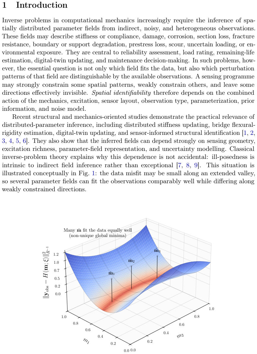
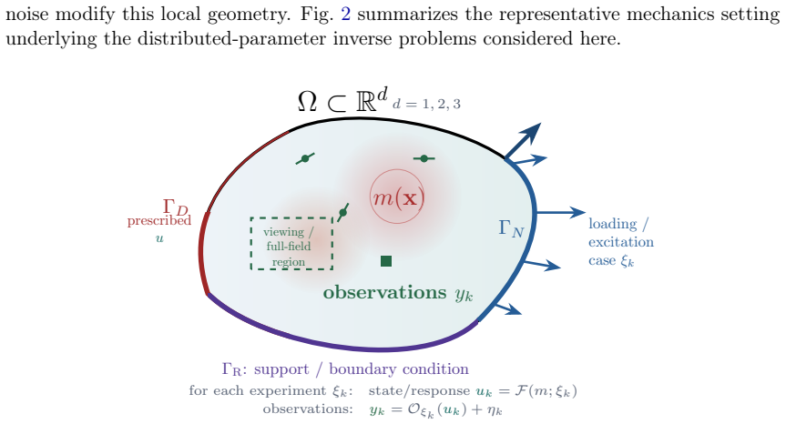
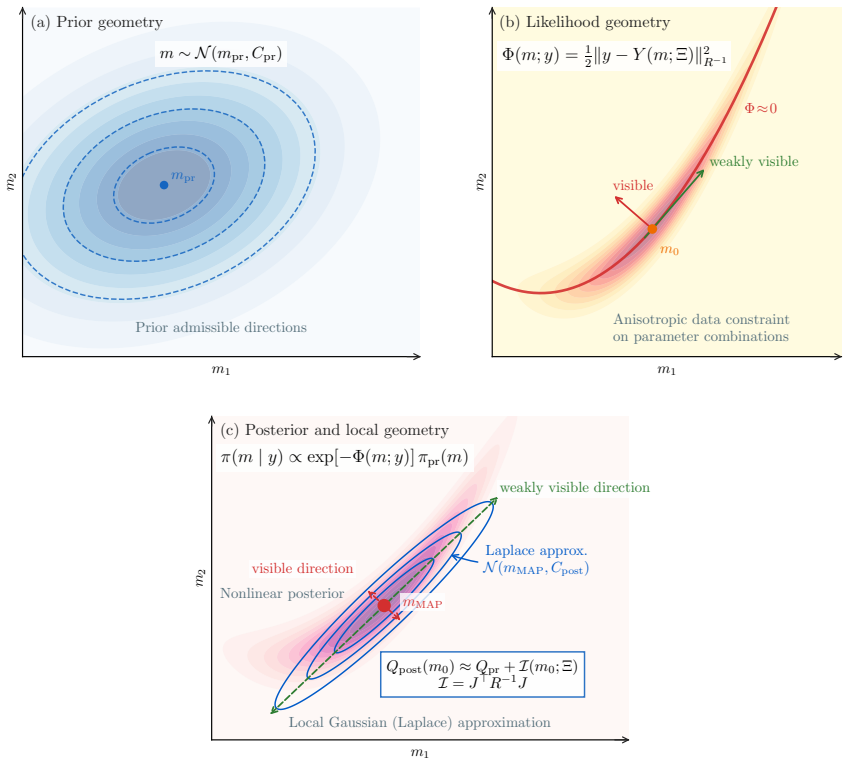
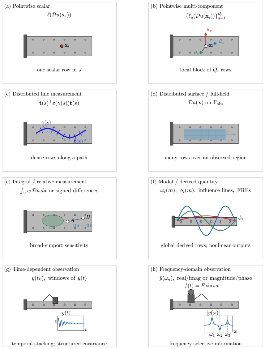
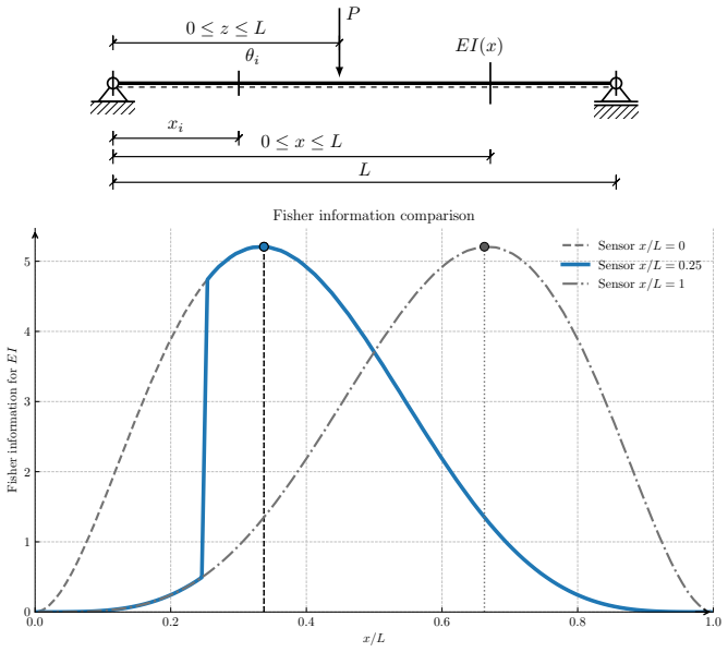
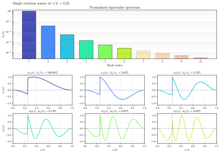
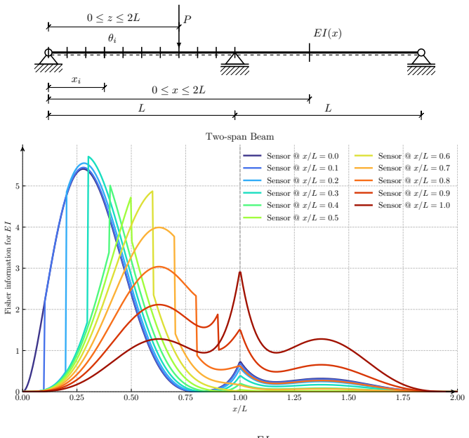
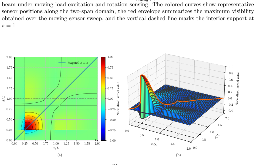
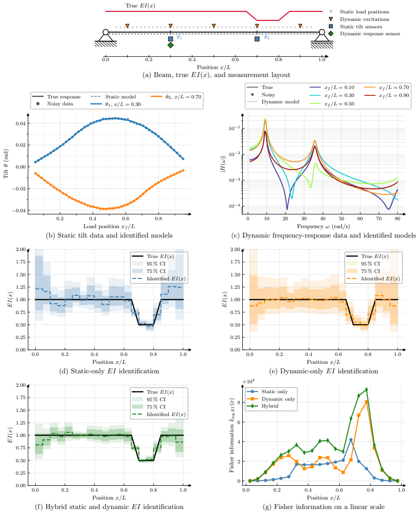
In distributed-parameter inverse problems in computational mechanics, spatially varying fields are inferred from noisy, indirect, and heterogeneous observations. The relevant identifiability question concerns which spatial perturbation patterns of the field are distinguishable under a specified sensing and excitation programme. This paper develops a local information-operator framework for this purpose. Around a nominal parameter field, the parameter-to-observation map is linearized and the likelihood contribution to posterior precision is interpreted as an operator on parameter-field perturbations. For locally linearized Gaussian models with parameter-independent covariance, this operator is equivalently Fisher information, Gauss-Newton data-misfit curvature, and a noise-weighted sensitivity Gramian. The framework separates pointwise visibility from spatial identifiability. The diagonal gives a coordinate-dependent local information density, while the full kernel and metric- or prior-preconditioned spectra rank spatial patterns that are strongly visible, weakly visible, or locally invisible. Heterogeneous observation blocks are assembled in a common parameter space; information is additive only under conditional independence, whereas correlated errors require the full joint covariance. Model discrepancy, nuisance parameters, and prior information modify the same geometry through covariance inflation, Schur-complement information loss, and prior-preconditioned modes. Examples cover analytic beam kernels, two-span support coupling, static-dynamic fusion for flexural-rigidity identification, and two-dimensional damage-field reconstruction in a leading information subspace. The operator view supports interpretation of identifiability, sensor complementarity, and reduced reconstruction in distributed-parameter inverse problems.
Editorial analysis
A structured set of objections, weighed in public.
Referee Report
Summary. The paper develops a local information-operator framework for spatial identifiability questions in distributed-parameter inverse problems. Around a nominal parameter field the parameter-to-observation map is linearized; the likelihood contribution to posterior precision is interpreted as an operator on field perturbations. Under the stated scope (locally linearized Gaussian models with parameter-independent covariance) this operator is equivalently the Fisher information, the Gauss-Newton data-misfit curvature, and the noise-weighted sensitivity Gramian. The diagonal supplies a coordinate-dependent local information density while the kernel and (metric- or prior-preconditioned) spectra rank strongly visible, weakly visible, or locally invisible spatial patterns. Heterogeneous observation blocks are assembled in a common parameter space; information additivity, model discrepancy, nuisance parameters, and priors are handled via standard Gaussian rules (conditional independence, covariance inflation, Schur complements). Analytic and numerical examples are given for beam kernels, two-span coupling, static-dynamic fusion, and 2-D damage-field reconstruction.
Significance. If the equivalences hold, the operator view supplies a compact, geometrically interpretable language for identifiability, sensor complementarity, and reduced reconstruction that is directly usable by practitioners in computational mechanics. The explicit reduction to standard second-derivative quantities of the Gaussian negative log-likelihood and the clean separation of pointwise versus pattern-wise visibility are the main contributions; the handling of heterogeneous blocks and prior preconditioning follows directly from existing information geometry and does not introduce new machinery.
minor comments (3)
- The abstract packs several distinct concepts (operator equivalences, diagonal/kernel decomposition, heterogeneous blocks, Schur complements) into a single paragraph; splitting the framework description into two or three shorter sentences would improve readability without changing content.
- Early in the manuscript an explicit equation defining the local information operator (e.g., as the integral kernel of the linearized map composed with the inverse covariance) would anchor the subsequent verbal descriptions.
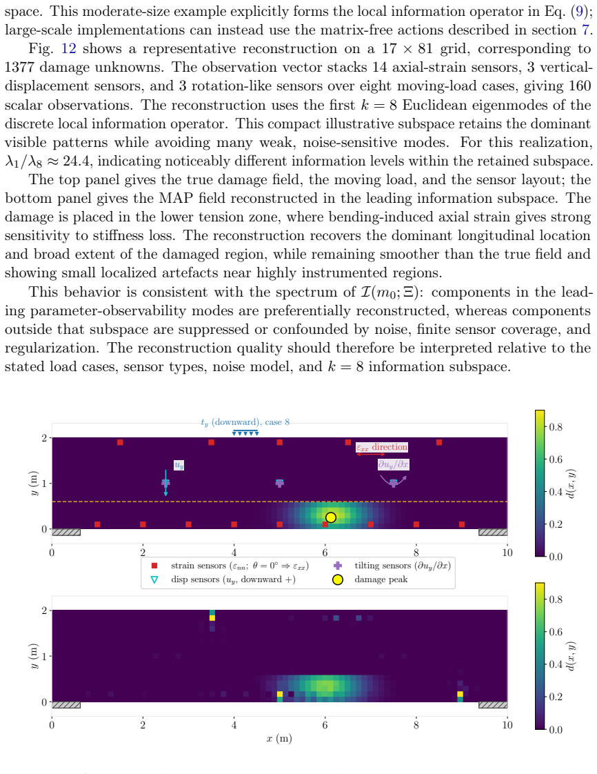
- In the examples section, the transition from the analytic beam kernels to the two-dimensional damage reconstruction would benefit from a short statement of the discretization size and the numerical linear-algebra method used to extract the leading eigenmodes.
Simulated Author's Rebuttal
We thank the referee for the thorough summary and positive evaluation of the local information-operator framework. The report correctly identifies the core contributions and the scope limitations (linearized Gaussian models with parameter-independent covariance). No specific major comments requiring point-by-point rebuttal were listed in the report.
Circularity Check
No significant circularity; equivalences follow from standard definitions
full rationale
The paper scopes its claims explicitly to locally linearized Gaussian models with parameter-independent covariance. Under these conditions the stated operator equivalences (Fisher information, Gauss-Newton data-misfit curvature, noise-weighted sensitivity Gramian) are direct algebraic consequences of the second derivative of the negative log-likelihood and the coincidence of the Gauss-Newton Hessian with the true Hessian for a linearized map; they do not reduce any claimed result to a fitted quantity defined by the result itself. The diagonal-versus-kernel decomposition is the standard spectral decomposition of a compact self-adjoint operator on the parameter space. No self-citation is invoked as load-bearing justification, no uniqueness theorem is imported from the authors' prior work, and no ansatz is smuggled in. The framework therefore remains self-contained against external benchmarks of information geometry and Gaussian inverse problems.
Axiom & Free-Parameter Ledger
axioms (2)
- domain assumption The parameter-to-observation map admits a linearization around a nominal field.
- domain assumption Observation covariance is independent of the parameter field.
invented entities (1)
-
Local information operator
no independent evidence
Reference graph
Works this paper leans on
-
[1]
Adhikari, S. and Friswell, M. I. Distributed Parameter Model Updating Using the Karhunen–Loève Expansion.Mechanical Systems and Signal Processing24.(2) (2010), 326–339.doi:10.1016/j.ymssp.2009.08.007
-
[2]
et al.High-Fidelity Digital Twins: Detecting and Localizing Weaknesses in Structures
Löhner, R. et al.High-Fidelity Digital Twins: Detecting and Localizing Weaknesses in Structures. 2023.doi:10.48550/arXiv.2311.10925. 35
-
[3]
Airaudo, F. N. et al. Adjoint-Based Determination of Weaknesses in Structures. Computer Methods in Applied Mechanics and Engineering417(2023), 116471.doi: 10.1016/j.cma.2023.116471
- [4]
-
[5]
Bakeer, T., Herbers, M., and Marx, S.Sensor Informativeness, Identifiability, and Uncertainty in Bayesian Inverse Problems for Structural Health Monitoring. 2025. doi:10.48550/arXiv.2511.16628
-
[6]
Diaz, M., Charbonnel, P.-É., and Chamoin, L. Merging Experimental Design and Structural Identification around the Concept of Modified Constitutive Relation Error in Low-Frequency Dynamics for Enhanced Structural Monitoring.Mechanical Systems and Signal Processing197(2023), 110371.doi:10.1016/j.ymssp.2023.110371
-
[7]
Beck, J. V. and Arnold, K. J.Parameter Estimation in Engineering and Science. New York: Wiley, 1977
1977
-
[8]
Philadelphia, PA: Society for Industrial and Applied Mathematics, 2005
Tarantola, A.Inverse Problem Theory and Methods for Model Parameter Estimation. Philadelphia, PA: Society for Industrial and Applied Mathematics, 2005
2005
-
[9]
Stuart, A. M. Inverse Problems: A Bayesian Perspective.Acta Numerica19(2010), 451–559.doi:10.1017/S0962492910000061
-
[10]
Kammer, D. C. Sensor Placement for On-Orbit Modal Identification and Correlation of Large Space Structures.Journal of Guidance, Control, and Dynamics14.(2) (1991), 251–259.doi:10.2514/3.20635
-
[11]
Sensor Placement for Parameter Estimation of Structures Using Fisher Information Matrix
Sanayei, M. and Javdekar, C. N. “Sensor Placement for Parameter Estimation of Structures Using Fisher Information Matrix”.Applications of Advanced Technologies in Transportation (2002). Boston Marriot, Cambridge, Massachusetts, United States: American Society of Civil Engineers, 2002, pp. 385–386.doi:10.1061/40632(245)49
-
[12]
Papadimitriou, C., Beck, J. L., and Au, S.-K. Entropy-Based Optimal Sensor Location for Structural Model Updating.Journal of Vibration and Control6.(5) (2000), 781– 800.doi:10.1177/107754630000600508
-
[13]
Papadimitriou, C. Optimal Sensor Placement Methodology for Parametric Identifica- tion of Structural Systems.Journal of Sound and Vibration278.(4) (2004), 923–947. doi:10.1016/j.jsv.2003.10.063
-
[14]
Yi, T.-H. and Li, H.-N. Methodology Developments in Sensor Placement for Health Monitoring of Civil Infrastructures.International Journal of Distributed Sensor Networks8.(8) (2012), 612726.doi:10.1155/2012/612726
-
[15]
Barthorpe, R. J. and Worden, K. Emerging Trends in Optimal Structural Health Monitoring System Design: From Sensor Placement to System Evaluation.Journal of Sensor and Actuator Networks9.(3) (2020), 31.doi:10.3390/jsan9030031
-
[16]
Ebrahimian, H. et al. Information-Theoretic Approach for Identifiability Assessment of Nonlinear Structural Finite-Element Models.Journal of Engineering Mechanics 145.(7) (2019), 04019039.doi:10.1061/(ASCE)EM.1943-7889.0001590
-
[17]
Ercan, T. and Papadimitriou, C. Bayesian Optimal Sensor Placement for Parameter Estimation under Modeling and Input Uncertainties.Journal of Sound and Vibration 563(2023), 117844.doi:10.1016/j.jsv.2023.117844. 36
-
[18]
2026.doi:10.48550/ arXiv.2602.02981
Antil, H., Jain, A., and Löhner, R.Fisher-Information-Based Sensor Placement for Structural Digital Twins: Analytic Results and Benchmarks. 2026.doi:10.48550/ arXiv.2602.02981
-
[19]
Vande Wouwer, A. et al. An Approach to the Selection of Optimal Sensor Locations in Distributed Parameter Systems.Journal of Process Control10.(4) (2000), 291–300. doi:10.1016/S0959-1524(99)00048-7
-
[20]
Huan, X. and Marzouk, Y. M. Simulation-Based Optimal Bayesian Experimental Design for Nonlinear Systems.Journal of Computational Physics232.(1) (2013), 288–317.doi:10.1016/j.jcp.2012.08.013
-
[21]
Alexanderian, A. et al. A-Optimal Design of Experiments for Infinite-Dimensional Bayesian Linear Inverse Problems with Regularizedℓ0-Sparsification.SIAM Journal on Scientific Computing36.(5) (2014), A2122–A2148.doi:10.1137/130933381
-
[22]
Alexanderian, A. Optimal Experimental Design for Infinite-Dimensional Bayesian Inverse Problems Governed by PDEs: A Review.Inverse Problems37.(4) (2021), 043001.doi:10.1088/1361-6420/abe10c
-
[23]
Ryan, E. G. et al. A Review of Modern Computational Algorithms for Bayesian Optimal Design.International Statistical Review84.(1) (2016), 128–154.doi: 10. 1111/insr.12107
2016
-
[24]
Optimal Experimental Design: Formu- lations and Computations.Acta Numerica33(2024), 715–840.doi: 10
Huan, X., Jagalur, J., and Marzouk, Y. Optimal Experimental Design: Formu- lations and Computations.Acta Numerica33(2024), 715–840.doi: 10 . 1017 / S0962492924000023
2024
-
[25]
Flath, H. P. et al. Fast Algorithms for Bayesian Uncertainty Quantification in Large- Scale Linear Inverse Problems Based on Low-Rank Partial Hessian Approximations. SIAM Journal on Scientific Computing33.(1) (2011), 407–432.doi: 10 . 1137 / 090780717
2011
-
[26]
Bui-Thanh, T. et al. A Computational Framework for Infinite-Dimensional Bayesian Inverse Problems Part I: The Linearized Case, with Application to Global Seismic Inversion.SIAM Journal on Scientific Computing35.(6) (2013), A2494–A2523.doi: 10.1137/12089586X
-
[27]
Cui, T. et al. Likelihood-Informed Dimension Reduction for Nonlinear Inverse Prob- lems.Inverse Problems30.(11) (2014), 114015.doi: 10.1088/0266-5611/30/11/ 114015
-
[28]
Spantini, A. et al. Optimal Low-rank Approximations of Bayesian Linear Inverse Problems.SIAM Journal on Scientific Computing37.(6) (2015), A2451–A2487.doi: 10.1137/140977308
-
[29]
Likelihood-informed Model Reduction for Bayesian Inference of Static Structural Loads
Scheffels, J. et al.Likelihood-Informed Model Reduction for Bayesian Inference of Static Structural Loads. 2025.doi:10.48550/arXiv.2510.07950
work page internal anchor Pith review Pith/arXiv arXiv doi:10.48550/arxiv.2510.07950 2025
-
[30]
Moore, B. Principal Component Analysis in Linear Systems: Controllability, Ob- servability, and Model Reduction.IEEE Transactions on Automatic Control26.(1) (1981), 17–32.doi:10.1109/TAC.1981.1102568
-
[31]
Scherpen, J. M. A. Balancing for Nonlinear Systems.Systems & Control Letters21.(2) (1993), 143–153.doi:10.1016/0167-6911(93)90117-O
-
[32]
Lall, S., Marsden, J. E., and Glavaški, S. Empirical Model Reduction of Controlled Nonlinear Systems.IFAC Proceedings Volumes. 14th IFAC World Congress 1999, Beijing, Chia, 5-9 July32.(2) (1999), 2598–2603.doi:10.1016/S1474- 6670(17) 56442-3. 37
-
[33]
emgr - The Empirical Gramian Framework.Algorithms11.(7) (2018), 91
Himpe, C. emgr - The Empirical Gramian Framework.Algorithms11.(7) (2018), 91. doi:10.3390/a11070091
-
[34]
Observability and Fisher Information Matrix in Nonlinear Regression
Jauffret, C. Observability and Fisher Information Matrix in Nonlinear Regression. IEEE Transactions on Aerospace and Electronic Systems43.(2) (2007), 756–759.doi: 10.1109/TAES.2007.4285368
-
[35]
Lewis, J. M. and Lakshmivarahan, S. Role of the Observability Gramian in Param- eter Estimation: Application to Nonchaotic and Chaotic Systems via the Forward Sensitivity Method.Atmosphere13.(10) (2022).doi:10.3390/atmos13101647
-
[36]
Kunwoo, L. et al. Observability Gramian for Bayesian Inference in Nonlinear Systems With Its Industrial Application.IEEE Control Systems Letters7(2023), 871–876. doi:10.1109/LCSYS.2022.3227452
-
[37]
The Bayesian Approach to Inverse Problems
Dashti, M. and Stuart, A. M. “The Bayesian Approach to Inverse Problems”.Handbook of Uncertainty Quantification. Cham: Springer, Cham, 2017, pp. 311–428.doi:10. 1007/978-3-319-12385-1_7
2017
-
[38]
Powel, N. and Morgansen, K. A.Empirical Observability Gramian for Stochastic Observability of Nonlinear Systems. 2020.doi:10.48550/arXiv.2006.07451
-
[39]
Boyacıoğlu, B. and van Breugel, F. Duality of Stochastic Observability and Con- structability and Links to Fisher Information.IEEE Control Systems Letters8(2024), 3458–3463.doi:10.1109/LCSYS.2025.3547297
-
[40]
Ashyraliyev, M. et al. Systems Biology: Parameter Estimation for Biochemical Models. The FEBS Journal276.(4) (2009), 886–902.doi:10.1111/j.1742-4658.2008.06844. x
-
[41]
Qi, J. and Baker, R. E. Optimal Experimental Design for Parameter Estimation in the Presence of Observation Noise.Mathematical Biosciences392(2026), 109571. doi:10.1016/j.mbs.2025.109571
-
[42]
Attia, A. and Constantinescu, E. Optimal Experimental Design for Inverse Problems in the Presence of Observation Correlations.SIAM Journal on Scientific Computing 44(2022).doi:10.1137/21M1418666
-
[43]
Petra, N. et al. A Computational Framework for Infinite-Dimensional Bayesian Inverse Problems, Part II: Stochastic Newton MCMC with Application to Ice Sheet Flow Inverse Problems.SIAM Journal on Scientific Computing36.(4) (2014), A1525– A1555.doi:10.1137/130934805
-
[44]
Cui, T., Tong, X. T., and Zahm, O. Prior Normalization for Certified Likelihood- Informed Subspace Detection of Bayesian Inverse Problems.Inverse Problems38.(12) (2022), 124002.doi:10.1088/1361-6420/ac9582
-
[45]
Bertola, N. J. et al. Optimal Multi-Type Sensor Placement for Structural Identification by Static-Load Testing.Sensors (Basel, Switzerland)17.(12) (2017), 2904.doi: 10.3390/s17122904
-
[46]
Bell, E. S. et al. Multiresponse Parameter Estimation for Finite-Element Model Updating Using Nondestructive Test Data.Journal of Structural Engineering133.(8) (2007), 1067–1079.doi:10.1061/(ASCE)0733-9445(2007)133:8(1067)
-
[47]
Kim, S. et al. A Sequential Framework for Improving Identifiability of FE Model Updating Using Static and Dynamic Data.Sensors19.(23) (2019), 5099.doi: 10. 3390/s19235099. 38
2019
-
[48]
Attia, A., Alexanderian, A., and Saibaba, A. K. Goal-Oriented Optimal Design of Experiments for Large-Scale Bayesian Linear Inverse Problems.Inverse Problems 34.(9) (2018).doi:10.1088/1361-6420/aad210
-
[49]
Kennedy, M. C. and O’Hagan, A. Bayesian Calibration of Computer Models.Journal of the Royal Statistical Society: Series B (Statistical Methodology)63.(3) (2001), 425–464.doi:10.1111/1467-9868.00294
-
[50]
and O’Hagan, A
Brynjarsdóttir, J. and O’Hagan, A. Learning about Physical Parameters: The Impor- tance of Model Discrepancy.Inverse Problems30.(11) (2014), 114007.doi: 10.1088/ 0266-5611/30/11/114007
2014
-
[51]
Ling, Y., Mullins, J., and Mahadevan, S. Selection of Model Discrepancy Priors in Bayesian Calibration.Journal of Computational Physics276(2014), 665–680.doi: 10.1016/j.jcp.2014.08.005
-
[52]
Alexanderian, A. et al. A Fast and Scalable Method for A-Optimal Design of Experi- ments for Infinite-dimensional Bayesian Nonlinear Inverse Problems.SIAM Journal on Scientific Computing38.(1) (2016), A243–A272.doi:10.1137/140992564
-
[53]
Sensor Placement on a Cantilever Beam Using Observability Gramians
Brace, N. L. et al. “Sensor Placement on a Cantilever Beam Using Observability Gramians”.2022 IEEE 61st Conference on Decision and Control (CDC). IEEE, 2022, pp. 388–395.doi:10.1109/CDC51059.2022.9992639
-
[54]
Bagheri, A. et al. Identification of Flexural Rigidity in Bridges with Limited Structural Information.Journal of Structural Engineering144.(8) (2018), 04018126.doi: 10. 1061/(ASCE)ST.1943-541X.0002131
2018
-
[55]
Koo, K.-Y. and Yi, J.-H. Substructural Identification of Flexural Rigidity for Beam- Like Structures.Shock and Vibration2015(2015), 1–15.doi: 10.1155/2015/726410
-
[56]
Lee, U. and Shin, J. A Frequency-Domain Method of Structural Damage Identification Formulated from the Dynamic Stiffness Equation of Motion.Journal of Sound and Vibration257.(4) (2002), 615–634.doi:10.1006/jsvi.2002.5058
- [57]
-
[58]
Bońkowski, P. A. et al. Stiffness Identification of Reinforced Concrete Beams Using Rotation Rate Sensors.Engineering Structures307(2024), 117969.doi: 10.1016/j. engstruct.2024.117969
work page doi:10.1016/j 2024
-
[59]
Qian, E. et al. Model Reduction of Linear Dynamical Systems via Balancing for Bayesian Inference.Journal of Scientific Computing91.(1) (2022), 29.doi: 10.1007/ s10915-022-01798-8
2022
-
[60]
Bangerth, W. et al. Estimating and Using Information in Inverse Problems.Inverse Problems and Imaging24(2026), 1–33.doi:10.3934/ipi.2026003
-
[61]
Menke, W.Resolution and Covariance in Generalized Least Squares Inversion. 2014
2014
-
[62]
Wieland, F.-G. et al. On Structural and Practical Identifiability.Current Opinion in Systems Biology25(2021), 60–69.doi:10.1016/j.coisb.2021.03.005
-
[63]
Huber, P. J. Robust Estimation of a Location Parameter.The Annals of Mathematical Statistics35.(1) (1964), 73–101.doi:10.1214/aoms/1177703732
-
[64]
Huber, P. J. and Ronchetti, E.Robust Statistics. 2nd ed. Wiley Series in Probability and Statistics. Hoboken, N.J: Wiley, 2009.doi:10.1002/9780470434697. 39
discussion (0)
Sign in with ORCID, Apple, or X to comment. Anyone can read and Pith papers without signing in.