REVIEW 2 major objections 3 minor 1 cited by
A Groupwise Approach for Inferring Heterogeneous Treatment Effects in Causal Inference
T0 review · 2 major / 3 minor · reviewed 2026-08-14 · deepseek-v4-flash
Pith's one-line read A sample-splitting least squares estimator estimates subgroup treatment effects directly, attains the semiparametric efficiency bound under homoskedastic errors, and stays valid when the propensity score is constant within subgroups even…
desk verdict A useful, honest paper on subgroup treatment effects; the reader's variance objection to Theorem 3.2 does not survive contact with the proof, but the unverified rate conditions for ML nuisance estimators are a real gap. read the letter →
The pith
A machine-rendered reading of the paper's core claim, the machinery that carries it, and where it could break.
The reading
What carries the argument
The load-bearing object is the SSLS estimator, a two-fold cross-fitted least squares estimator built on the Robinson transformation. For groupwise effects the transformed model is $Y_i-\mathbb{E}(Y_i|X_i)=\{A_i-e(X_i)\}\mathbf{I}(X_i)^\top\tau+\epsilon_i$, so SSLS fits the nuisance functions $\mathbb{E}(Y_i|X_i)$ and $e(X_i)$ on one subsample and runs least squares of the residualized outcome on the residualized subgroup dummies in the other. The identity that carries the argument is that SSLS is an unregularized special case of the R-learner, and cross-fitting plus fast nuisance convergence makes it behave like the oracle least squares estimator with covariance $\Sigma=E[\{A_i-e(X_i)\}^2\mathbf{I}(X_i)\mathbf{I}(X_i)^\top]^{-1}E[\epsilon_i^2\{A_i-e(X_i)\}^2\mathbf{I}(X_i)\mathbf{I}(X_i)^\top](\cdots)^{-1}$. The diagonal structure comes from disjoint subgroup indicators and is what makes the Sidak/maxT simultaneous inference exact in the Gaussian limit.
What would settle it
Simulate a correctly specified, homoskedastic data-generating process satisfying Assumption 3.1, estimate the nuisances with an oracle and then with a slow-converging learner such as a shallow tree, and compare the empirical standard error of $\hat{\tau}_{\mathrm{SSLS}}$ to the claimed diagonal covariance: if the slow-learner intervals undercover markedly while the oracle intervals achieve nominal coverage, the fast-rate assumption is the load-bearing part of the theorem.
Extended reading notes
Core claim
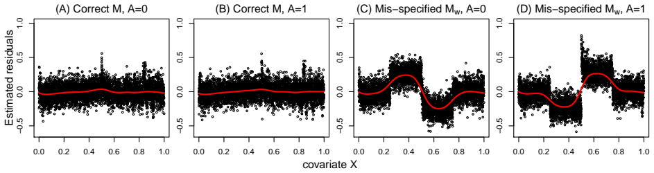
On the paper's own terms, the central discovery is that the groupwise treatment effect vector $\tau=(\tau_1,\ldots,\tau_G)$ can be estimated directly at the semiparametric efficiency bound by ordinary least squares after the Robinson transformation, subtracting $\mathbb{E}(Y_i|X_i)$ from the outcome and $e(X_i)$ from the treatment and regressing the residualized outcome on the residualized subgroup indicators $\{A_i-e(X_i)\}\mathbf{I}(X_i)$. Under Assumption 3.1, $\sqrt{N}(\hat{\tau}_{\mathrm{SSLS}}-\tau)\xrightarrow{d}N(0,\Sigma)$ with diagonal $\Sigma$; under homoskedastic errors $\Sigma$ is the semiparametric variance lower bound. If model (7) is misspecified but the propensity score $e(X_i)$ is constant within each subgroup, the same estimator still converges to the true subgroup average effects, though not at the efficiency bound. The paper also establishes that data-driven groupings $M$ learned by clustering on one third of the data preserve asymptotic Normality when the clustering is consistent, and it supplies simultaneous max-statistic inference, a residual diagnostic for misspecified $M$, and an application to a 1.88-million-voter field experiment.
Load-bearing premise
The load-bearing premise is that the machine-learned nuisance estimates for $\mathbb{E}(Y_i|X_i)$ and $e(X_i)$ converge fast enough—specifically $\sqrt{N}\|\hat{e}-e\|^2_{P,2}\to 0$ and the analogous product rate—and these fast rates are not formally established for the boosted trees and neural networks the paper uses in its simulations and data analysis.
Editorial extensions
If this is right
- Directly estimating $\tau_g$ can beat a two-step approach that estimates $\tau(x)$ with a generalized random forest and then averages within subgroups; in the paper's simulations SSLS has smaller bias, smaller variance, and higher power.
- Finer partitions are generally less efficient: the asymptotic variance of $\hat\tau_g$ grows as the subgroup shrinks, so subgroup definitions should balance interpretability with sample size.
- When the propensity score is constant within each subgroup, as in a completely randomized experiment, SSLS remains consistent and asymptotically Normal for $\tau_g$ even if the linear subgroup model (7) is misspecified.
- If $M$ is chosen by clustering, splitting the data into three parts—one for clustering, two for SSLS—preserves asymptotic Normality provided the clustering converges to the true groups at the required rate.
- Simultaneous confidence statements across all subgroups can use the maxT/Sidak critical value, because the estimated subgroup effects are asymptotically independent.
Reading between the lines
- A natural extension would be to test whether the efficiency claim survives heteroskedastic errors; the proof marks homoskedasticity as the point where the diagonal variance becomes the semiparametric lower bound, so simulations varying within-subgroup error variance would quantify the gap.
- Because the fast convergence rates in Assumption 3.1(c) are not verified for the boosted trees and neural networks used in the paper's own Section 4, a cautious reader should treat those confidence intervals as approximate unless the rates are checked or nuisance estimators with known rates are used.
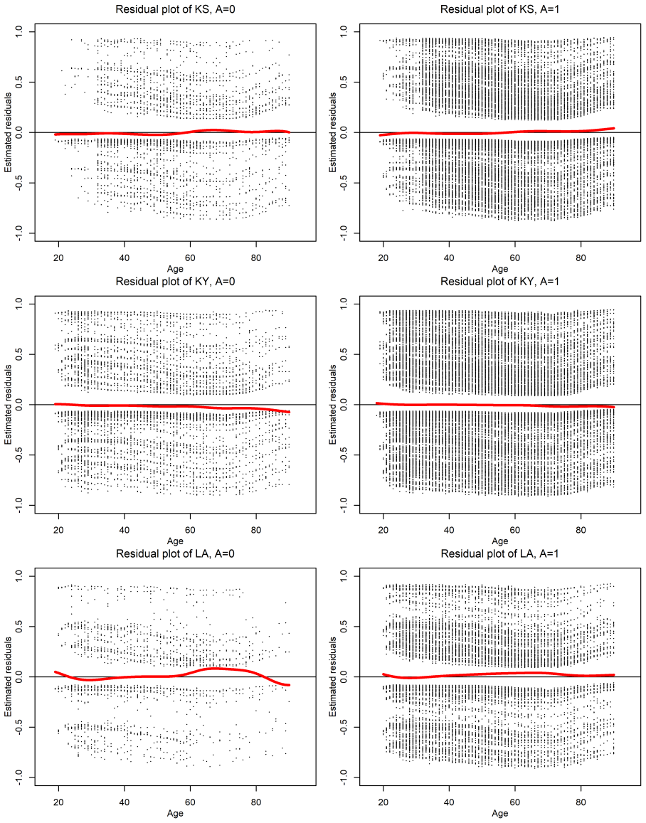
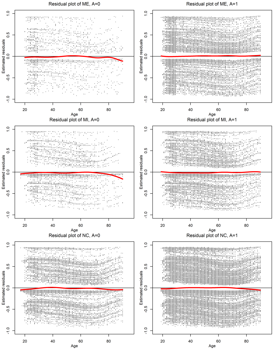
- The residual diagnostic suggests a model-selection routine: search over candidate groupings and keep the coarsest one whose SSLS residuals satisfy the mean-zero condition; post-selection inference after such a search is not analyzed here.
- The R-learner connection implies the efficiency result may extend to other low-dimensional linear functionals of the CATE estimated by cross-fitted least squares, not just subgroup indicators.
Signed reviews
Editorial analysis
A structured set of objections, weighed in public.
Referee Report
Summary. The paper proposes a 'sample splitting least squares' (SSLS) estimator for groupwise average treatment effects. After cross-fitting estimates of the propensity score and the conditional outcome mean, the method runs a linear regression of the residualized outcome on residualized subgroup indicators. The authors prove asymptotic normality of the estimator, show that it attains the semiparametric efficiency bound under homoskedastic errors, and provide a robustness result: under misspecification of the treatment-effect model, the estimator remains consistent and asymptotically normal provided the propensity score is constant within each subgroup. The paper also extends the procedure to data-driven subgroup choice via clustering, proposes simultaneous inference based on the max statistic, and reports simulations and a reanalysis of a large voter-turnout experiment.
Significance. If the results hold, this is a useful and practical contribution: it packages cross-fitted regression into a simple, interpretable tool for effect heterogeneity over pre-defined subgroups, explicitly connects to the R-learner, and gives a clean condition under which the estimator is robust to model misspecification. The proofs are detailed and follow standard semiparametric cross-fitting arguments; the efficiency calculation in the supplementary material is careful. The robustness result in Theorem 3.2 and the variance plug-in for that setting are correct: contrary to the reader's concern, the residual under model (9) converges to (A-e)δ+epsilon, so the plug-in estimator converges to Sigma' as derived in B.6. The main weakness is that the practical recommendation to use boosted trees and neural networks for nuisance functions is not covered by the formal assumptions, and the data analysis uses a median-aggregation procedure whose distribution is not derived.
major comments (2)
- [Assumption 3.1(c); Sections 4.1 and 5.2; Supplementary D] Assumption 3.1(c) requires sqrt(N) times the squared L2 error of the propensity score to vanish and sqrt(N) times the product of the propensity-score and outcome-regression errors to vanish. The paper nonetheless recommends boosted trees and neural networks for the nuisance fits, and Supplementary D states that rates for these methods are 'unknown and difficult to characterize.' Thus the headline claim that SSLS can incorporate flexible machine learning 'without sacrificing efficiency' is not formally established for the recommended implementation. Please either restrict the claim to learners satisfying Assumption 3.1(c), provide a concrete learner class with verified rates, or move the caveat into the main text and temper the conclusion accordingly.
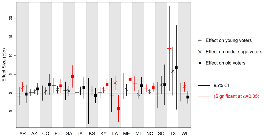
- [Section 5.2] The data analysis repeats SSLS 1,000 times and takes the median of the estimates, but no distribution theory is provided for this median. The asymptotic results in Section 3 apply to a single cross-fitted estimate from one split; the confidence intervals and p-values in Table 5 are therefore not formally justified for the median-aggregated estimator. Please either use a single split, provide a distributional result for the aggregation scheme, or clearly label the median procedure as a heuristic whose inferential properties are not covered by the theorems.
minor comments (3)
- [Section 5.2] The sentence 'since the propensity score in each subgroup is constant, the results about the SSLS estimator tau-hat_SSLS established in Theorem 3.1 holds even if model (7) is incorrect' should cite Theorem 3.2, which is the misspecification result; Theorem 3.1 assumes model (7).
- [Supplementary Table 2] In Table 2 of the supplementary materials, the column headers read 'sigma_A = 0, sigma_A = 1, sigma_A = 0'; the third block should be 'sigma_A = 2'.
- [Section 4.1, Table 1] The simulation discussion would benefit from an explanation of why boosted trees maintain near-nominal coverage under intra-cluster correlation while the oracle and SLNN estimators deteriorate sharply; as it stands, the robustness claim rests on a single simulation scenario.
Circularity Check
No significant circularity: the SSLS theorems follow from explicit assumptions and standard semiparametric theory, and no fitted parameter is renamed as a prediction.
full rationale
The paper's derivation chain is self-contained in the relevant sense. Theorems 2.2 and 2.3 are proved from explicit high-level conditions using standard cross-fitting and least-squares arguments, with full proofs in the supplementary materials; Theorems 3.1 and 3.2 are then applications of these general results to the Robinson-transformed model, with f* and g* explicitly defined. The target tau_g is defined as a subgroup average effect, and Theorem 3.2 verifies consistency under constant propensity by checking the moment condition E(epsilon' V*)=0 from the definition of tau_g, which is an identification step rather than a circular re-use of the conclusion. The paper openly identifies its estimator as a special case of the R-learner and cites external sources for cross-fitting, the Robinson transformation, and semiparametric efficiency bounds; there are no load-bearing self-citations, no imported uniqueness theorems, and no fitted constants presented as predictions. The rate conditions in Assumption 3.1(c) are assumptions, and the supplementary materials explicitly state that rates for boosted trees and neural networks are 'unknown and difficult to characterize'; this is a limitation in the coverage of the asymptotic guarantees, not a circular derivation.
Assumptions & free parameters
assumptions (5)
- domain assumption Causal identifying assumptions (A1) unconfoundedness, (A2) overlap, (A3) SUTVA
- domain assumption Homoskedastic errors E(ϵ²|V) = σ² for the semiparametric efficiency claim
- ad hoc to paper Fast nuisance convergence rates in Assumption 3.1(c): √N||ê-e||² → 0 and √N||ê-e||·||Ê-E|| → 0
- domain assumption Constant propensity score within each subgroup for Theorem 3.2
- ad hoc to paper Clustering consistency in Assumption 3.2: ||I{M̂≠M}||_P,2 → 0 and product rate with propensity score
Cite this review
Pith. "Pith review of A Groupwise Approach for Inferring Heterogeneous Treatment Effects in Causal Inference." pith.science (2026). https://pith.science/paper/7E3RTOXW
@misc{pith2026190804427,
  author       = {Pith},
  title        = {Pith review of: A Groupwise Approach for Inferring Heterogeneous Treatment Effects in Causal Inference},
  year         = {2026},
  howpublished = {\url{https://pith.science/paper/7E3RTOXW}},
  note         = {Machine review of arXiv:1908.04427}
}
read the original abstract
Recently, there has been great interest in estimating the conditional average treatment effect using flexible machine learning methods. However, in practice, investigators often have working hypotheses about effect heterogeneity across pre-defined subgroups of study units, which we call the groupwise approach. The paper compares two modern ways to estimate groupwise treatment effects, a nonparametric approach and a semiparametric approach, with the goal of better informing practice. Specifically, we compare (a) the underlying assumptions, (b) efficiency and adaption to the underlying data generating models, and (c) a way to combine the two approaches. We also discuss how to test a key assumption concerning the semiparametric estimator and to obtain cluster-robust standard errors if study units in the same subgroups are correlated. We demonstrate our findings by conducting simulation studies and reanalyzing the Early Childhood Longitudinal Study.
Figures

Figures from the paper (5 more)



Forward citations
Cited by 1 Pith paper
-
Detecting Heterogeneous Treatment Effect with Instrumental Variables
A matched-pair instrumental variables method using CART on absolute adjusted outcome differences and closed testing discovers and tests heterogeneous complier treatment effects with familywise error control.
Reference graph
Works this paper leans on
-
[1]
Anderson, T. W. (2003) An Introduction to Multivariate Statistical Analysis. New York: Wiley, 3 edn
work page 2003
-
[2]
Arkansas Secretary of State, Little Rock
Arkansas Secretary of State (2017) Historical initiatives & referendum election results. Arkansas Secretary of State, Little Rock. (Available from https://www.sos.arkansas.gov/uploads/elections/Initiatives_and_Amendments_1938-2018.pdf.)
work page 2017
-
[3]
Athey, S. and Imbens, G. (2016) Recursive partitioning for heterogeneous causal effects. Proceedings of the National Academy of Sciences, 113, 7353--7360
work page 2016
-
[4]
Athey, S., Tibshirani, J. and Wager, S. (2019) Generalized random forests. The Annals of Statistics, 47, 1148--1178
work page 2019
-
[5]
Bickel, P. J., Klaassen, C. A., Ritov, Y. and Wellner, J. A. (1998) Efficient and adaptive estimation for semiparametric models. New York: Springer, 1 edn
work page 1998
-
[6]
Cai, T. T., Low, M. and Ma, Z. (2014) Adaptive confidence bands for nonparametric regression functions. Journal of the American Statistical Association, 109, 1054--1070
work page 2014
-
[7]
Chernozhukov, V., Chetverikov, D., Demirer, M., Duflo, E., Hansen, C., Newey, W. and Robins, J. (2018) Double/debiased machine learning for treatment and structural parameters. The Econometrics Journal, 21, C1--C68
work page 2018
-
[8]
Chernozhukov , V., Demirer , M., Duflo , E. and Fernandez-Val , I. (2017) Generic machine learning inference on heterogenous treatment effects in randomized experiments . Preprint arXiv:1712.04802. Department of Economics, Massachusetts Institute of Technology, Cambridge
arXiv 2017
Show all 48 references
-
[9]
and Miratrix, L
Ding, P., Feller, A. and Miratrix, L. (2019) Decomposing treatment effect variation. Journal of the American Statistical Association, 114, 304--317
2019
-
[10]
and Cervone, D
Dorie, V., Hill, J., Shalit, U., Scott, M. and Cervone, D. (2019) Automated versus do-it-yourself methods for causal inference: Lessons learned from a data analysis competition. Statistical Science, 34, 43--68
2019
-
[11]
Dunn, O. J. (1958) Estimation of the means of dependent variables. The Annals of Mathematical Statistics, 29, 1095--1111
1958
-
[12]
Florida Department of State, Tallahassee
Florida Department of State (2019) Initiatives / amendments / revisions database. Florida Department of State, Tallahassee. (Available from https://dos.elections.myflorida.com/initiatives/.)
2019
-
[13]
Friedman, J. H. (2001) Greedy function approximation: A gradient boosting machine. The Annals of Statistics, 29, 1189--1232
2001
-
[14]
and Wasserman, L
Genovese, C. and Wasserman, L. (2008) Adaptive confidence bands. The Annals of Statistics, 36, 875--905
2008
-
[15]
S., Huber, G
Gerber, A. S., Huber, G. A., Fang, A. H. and Gooch, A. (2017) The generalizability of social pressure effects on turnout across high-salience electoral contexts: Field experimental evidence from 1.96 million citizens in 17 states. American Politics Research, 45, 533--559
2017
-
[16]
Gower, J. and J. S. Ross, G. (1969) Minimum spanning trees and single link cluster analysis. Journal of the Royal Statistical Society: Series C (Applied Statistics), 18, 54--64
1969
-
[17]
Gower, J. C. (1967) A comparison of some methods of cluster analysis. Biometrics, 23, 623--637
1967
-
[18]
R., Murray, J
Hahn, P. R., Murray, J. S. and Carvalho, C. M. (2020) Bayesian regression tree models for causal inference: Regularization, confounding, and heterogeneous effects (with discussion). Bayesian Analysis, 15, 965--1056
2020
-
[19]
and Friedman, J
Hastie, T., Tibshirani, R. and Friedman, J. (2009) The elements of statistical learning: data mining, inference and prediction. New York: Springer, 2 edn
2009
-
[20]
Hern\'an, M. A. and Robins, J. M. (2020) Causal Inference: What If. Boca Raton: Chapman & Hall/CRC
2020
-
[21]
Hill, J. L. (2011) Bayesian nonparametric modeling for causal inference. Journal of Computational and Graphical Statistics, 20, 217--240
2011
-
[22]
Y., Small, D
Hsu, J. Y., Small, D. S. and Rosenbaum, P. R. (2013) Effect modification and design sensitivity in observational studies. Journal of the American Statistical Association, 108, 135--148
2013
-
[23]
Y., Zubizarreta, J
Hsu, J. Y., Zubizarreta, J. R., Small, D. S. and Rosenbaum, P. R. (2015) Strong control of the familywise error rate in observational studies that discover effect modification by exploratory methods . Biometrika, 102, 767--782
2015
-
[24]
and Ratkovic, M
Imai, K. and Ratkovic, M. (2013) Estimating treatment effect heterogeneity in randomized program evaluation. The Annals of Applied Statistics, 7, 443--470
2013
-
[25]
Imbens, G. W. and Rubin, D. B. (2015) Causal Inference for Statistics, Social, and Biomedical Sciences: An Introduction. New York: Cambridge University Press
2015
-
[26]
(1995) A study of cross-validation and bootstrap for accuracy estimation and model selection
Kohavi, R. (1995) A study of cross-validation and bootstrap for accuracy estimation and model selection. In Proceedings of the 14th International Joint Conference on Artificial Intelligence, vol. 2, 1137--1143. San Francisco: Morgan Kaufmann Publishers Inc
1995
-
[27]
(2008) Building predictive models in r using the caret package
Kuhn, M. (2008) Building predictive models in r using the caret package. Journal of Statistical Software, Articles, 28, 1--26
2008
-
[28]
R., Sekhon, J
K \"u nzel, S. R., Sekhon, J. S., Bickel, P. J. and Yu, B. (2019) Meta-learners for estimating heterogeneous treatment effects using machine learning. Proceedings of the National Academy of Sciences, 116, 4156--4165
2019
-
[29]
Lee, K., Small, D. S. and Rosenbaum, P. R. (2018) A powerful approach to the study of moderate effect modification in observational studies. Biometrics, 74, 1161--1170
2018
-
[30]
(1957) Least squares quantization in PCM
Lloyd , S. (1957) Least squares quantization in PCM . Tech. rep., Bell Laboratories. Publisheed in 1982 in IEEE Transactions on Information Theory, 28(2):129--137
1957
-
[31]
Low, M. G. (1997) On nonparametric confidence intervals. The Annals of Statistics, 25, 2547--2554
1997
-
[32]
and Ben-David, S
von Luxburg, U. and Ben-David, S. (2005) Towards a statistical theory of clustering. Fraunhofer IPSI, Darmstadt, Germany. (Available from http://citeseerx.ist.psu.edu/viewdoc/download?doi=10.1.1.534.3125&rep=rep1&type=pdf.)
2005
-
[33]
(1967) Some methods for classification and analysis of multivariate observations
MacQueen, J. (1967) Some methods for classification and analysis of multivariate observations. In Proceedings of the Fifth Berkeley Symposium on Mathematical Statistics and Probability, Volume 1: Statistics, 281--297. Berkeley: University of California Press
1967
-
[34]
Newey, W. K. (1990) Semiparametric efficiency bounds. Journal of Applied Econometrics, 5, 99--135
1990
-
[35]
and Wager, S
Nie, X. and Wager, S. (2020) Quasi-Oracle Estimation of Heterogeneous Treatment Effects . Biometrika. Asaa076
2020
-
[36]
(1981) Strong consistency of k -means clustering
Pollard, D. (1981) Strong consistency of k -means clustering. The Annals of Statistics, 9, 135--140
1981
-
[37]
Robinson, P. M. (1988) Root-n-consistent semiparametric regression. Econometrica, 56, 931--954
1988
-
[38]
Rosenbaum, P. R. and Rubin, D. B. (1983) The central role of the propensity score in observational studies for causal effects. Biometrika, 70, 41--55
1983
-
[39]
Rubin, D. B. (1976) Inference and missing data. Biometrika, 63, 581--592
1976
-
[40]
The Annals of Statistics, 6, 34--58
--- (1978) Bayesian inference for causal effects: The role of randomization. The Annals of Statistics, 6, 34--58
1978
-
[41]
Shalit, U., Johansson, F. D. and Sontag, D. (2017) Estimating individual treatment effect: Generalization bounds and algorithms. In Proceedings of the 34th International Conference on Machine Learning, vol. 70 of Proceedings of Machine Learning Research, 3076--3085. JMLR.org
2017
-
[42]
(1973) SLINK: An optimally efficient algorithm for the single-link cluster method
Sibson, R. (1973) SLINK: An optimally efficient algorithm for the single-link cluster method . The Computer Journal, 16, 30--34
1973
-
[43]
(1967) Rectangular confidence regions for the means of multivariate normal distributions
Sidak, Z. (1967) Rectangular confidence regions for the means of multivariate normal distributions. Journal of the American Statistical Association, 62, 626--633
1967
-
[44]
Stone, C. J. (1980) Optimal rates of convergence for nonparametric estimators. The Annals of Statistics, 8, 1348--1360
1980
-
[45]
Su, X., Tsai, C.-L., Wang, H., Nickerson, D. M. and Li, B. (2009) Subgroup analysis via recursive partitioning. The Journal of Machine Learning Research, 10, 141--158
2009
-
[46]
(2005) Applied linear regression
Weisberg, S. (2005) Applied linear regression. Hoboken: Wiley-Interscience
2005
-
[47]
Wooldridge, J. M. (2010) Econometric Analysis of Cross Section and Panel Data. Cambridge: MIT press
2010
-
[48]
Zhao, Q., Small, D. S. and Ertefaie, A. (2017) Selective inference for effect modification via the lasso. Preprint arXiv:1705.08020. Department of Statistics, University of Pennsylvania, Philadelphia
2017 arXiv
Reviewed August 14, 2026 · model on record in the stance chip above.
Discussion (0). Continue with ORCID to comment.