REVIEW 3 major objections 5 minor 41 references
A New Approach for Constraining Large-Scale Temperature Fluctuations in the Intergalactic Medium
T0 review · 3 major / 5 minor · reviewed 2026-08-10 · deepseek-v4-flash
Pith's one-line read Quasar spectra cap IGM temperature swings at 100 Mpc scales to below 30 percent
desk verdict A careful new null measurement of IGM temperature fluctuations during helium reionization, but the headline upper limit depends on an unverified 100 Mpc coherence assumption that the authors themselves flag. read the letter →
The pith
A machine-rendered reading of the paper's core claim, the machinery that carries it, and where it could break.
The reading
What carries the argument
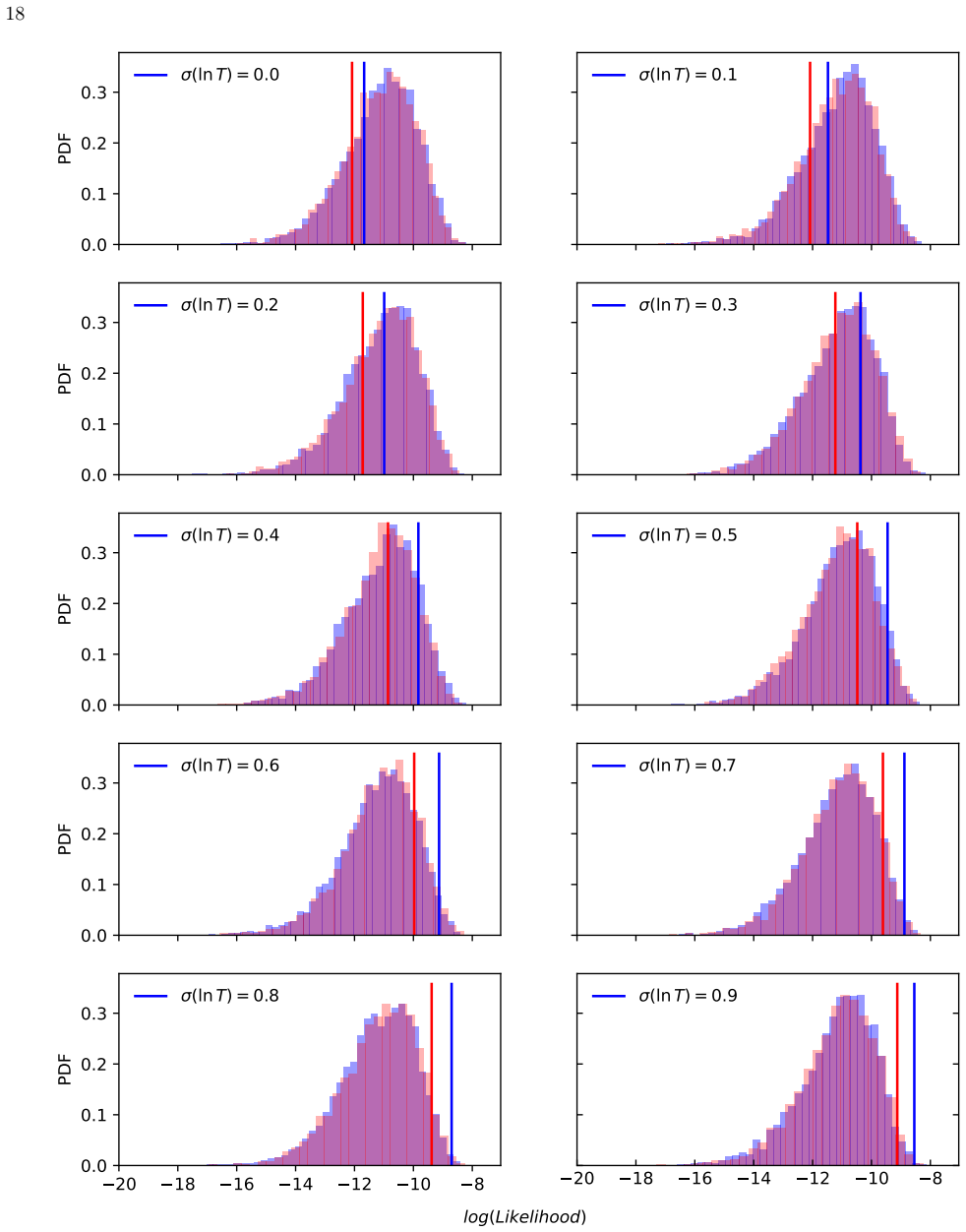
The central object is the distribution of effective Lyman-$\alpha$ optical depths, tau_eff, measured in 100 Mpc (and 50 Mpc) bins along 71 quasar sightlines. The mechanism is the temperature-opacity relation: hotter gas recombines more slowly, so a higher IGM temperature lowers the Lyman-$\alpha$ effective optical depth, and coherent large-scale temperature fluctuations rescale whole sightlines, broadening the observed tau_eff distribution beyond what the density field alone produces. The argument is carried by a lognormal temperature-fluctuation model in which each simulated sightline is rescaled by $\Delta$ ln tau = -0.352 $\Delta$ ln T, using the Bolton et al. (2005) calibration tau_eff proportional to $T^{0}$.352, followed by forward modeling that adds instrumental noise, continuum uncertainty, and a mean-flux calibration.
What would settle it
A measurement that would settle the claim is a comparison at z=3.76 on 100 Mpc scales using several hundred independent quasar sightlines with known continuum uncertainties: if the observed tau_eff distribution remains consistent with the no-fluctuation simulation, the sigma(ln T) < 0.29 limit is confirmed; if the distribution shows excess width beyond the density-only prediction, the limit is falsified. A second decisive test is a direct simulation of helium reionization with full radiative transfer that predicts a coherent temperature contrast above 30 percent at z=3.76; if such a model reproduces the observed narrow optical depth distribution, then the paper's temperature-opacity mapping is wrong rather than the temperature contrast being small.
Extended reading notes
Core claim
At redshift z=3.76, on 100 comoving Mpc scales, the rms large-scale temperature fluctuation of the intergalactic medium is constrained to $\sigma$(ln T) < 0.29 at 2 $\sigma$ (and < 0.40 at 3 $\sigma$), corresponding to a temperature contrast between ionized and neutral regions of roughly $\Delta$ T / T ~ 34% (49%). The observed effective optical depth distribution is consistent within 2 $\sigma$ with a cosmological hydrodynamical simulation that includes no temperature fluctuations, and the limits weaken at higher redshifts (z=3.90: <0.32; z=4.04: <0.74; z=4.19: <0.64 at 2 $\sigma$) because fewer sightlines are available. The paper concludes that either helium reionization had not yet imprinted temperature contrasts larger than roughly 30 percent at z=3.76, or the process had not significantly started at that redshift.
Load-bearing premise
The argument assumes that a large-scale temperature fluctuation acts as a coherent, sightline-wide rescaling of the effective optical depth with tau_eff proportional to $T^{0}$.352, whereas real helium reionization produces temperature fluctuations that are density-dependent, spatially structured, and also alter the temperature-density relation.
Editorial extensions
If this is right
- If the central claim holds, helium reionization's large-scale temperature contrast at z=3.76 is at most about 30 percent, ruling out the most extreme heating scenarios at that epoch.
- The effective optical depth distribution is a competitive and much simpler probe than the Lyman-alpha forest power spectrum for constraining reionization-induced temperature fluctuations.
- Roughly 400 to 700 quasar sightlines of similar quality would be needed to reach 2 sigma sensitivity to sigma(ln T) = 0.1, which would probe the temperature fluctuations predicted during most of helium reionization.
- The same method would be sensitive to any physical process that adds large-scale fluctuations to quantities modifying Lyman-alpha opacity, such as UV background fluctuations or the matter distribution.
- The tentative preference for non-zero temperature fluctuations at z=4.04 and z=4.19, if confirmed with larger samples, could indicate the onset of helium reionization at z > 4.
Reading between the lines
- The quoted upper limit on sigma(ln T) is only as strong as the coherence assumption; real helium reionization produces density-dependent, spatially structured temperature fields, so the limit should be read as constraining the coherent part of the temperature contrast rather than the total physical contrast.
- Because the same statistic is sensitive to any large-scale opacity fluctuation, the null result can be read as a consistency check of the standard cosmological model and of the UV background model used in the simulations.
- A testable extension would repeat the measurement on the much larger, lower signal-to-noise samples from DESI, WEAVE-QSO, and 4MOST, where the reduced continuum precision and increased noise are the main challenges to overcome.
- The scaling estimate sigma(ln T) ~ 1/sqrt(N_qso) suggests that pushing the same method to higher redshift with more sightlines could distinguish between a late-start and a low-contrast helium reionization history.
Editorial analysis
A structured set of objections, weighed in public.
Referee Report
Summary. This paper introduces a new method to constrain large-scale IGM temperature fluctuations during helium reionization by measuring the distribution of effective Lyman-α optical depths toward 71 quasars from the XQ-100 survey at z ≈ 3.76–4.19. The observed distributions are compared to Nyx hydrodynamical simulations with no temperature fluctuations, and the simulations are then post-processed to include coherent, lognormal temperature offsets per sightline with amplitude σ(ln T). The central result is an upper limit σ(ln T) < 0.29 (0.40 at 3σ) at z = 3.76 for 100 comoving Mpc averaging, with weaker constraints at higher redshifts and at 50 Mpc. The authors interpret this as implying that helium reionization had not imprinted temperature contrasts larger than about 30% at z = 3.76, or that it had not yet significantly started.
Significance. The measurement is carefully executed: the PCA continuum reconstruction has quantified accuracy, the sample is restricted to a flux-calibration-safe wavelength range, DLAs and bad pixels are masked, bootstrap resampling is used for uncertainties, and the simulations are forward-modeled with instrumental noise and continuum errors. The no-fluctuation model matches the observed cumulative distributions within 2σ, and the new statistic (the distribution of effective optical depths) is shown to have constraining power comparable to forecasts from power-spectrum analyses. If the model-dependent interpretation is validated, this would be the tightest constraint to date on large-scale temperature fluctuations from helium reionization. However, the physical interpretation relies on the assumption that temperature fluctuations are coherent over the sightline length and that the adopted τeff ∝ T^0.352 mapping captures the relevant physics; the paper itself labels the model 'rather simplistic,' which limits the astrophysical conclusion.
major comments (3)
- [§3.5.1, Table 3, abstract] The headline limit σ(ln T) < 0.29 is derived for a model in which each 100 Mpc sightline receives a single coherent lognormal temperature offset. If real helium reionization temperature fluctuations have a shorter coherence length, a given local temperature contrast produces less sightline-to-sightline scatter in τeff, so the same data allow larger physical temperature contrasts. The paper's own Table 3 shows the 2σ limit degrades from <0.29 at 100 Mpc to <0.40 at 50 Mpc, and the degradation continues for shorter coherence lengths approximately as sqrt(L/L_c). Section 5 concedes the fluctuations are 'unlikely to be so solidly coherent' but does not quantify the effect. The abstract's conclusion that the IGM temperature contrast is 'less than ~30%' is therefore not robust to finite coherence. Please either restrict the physical interpretation to the coherent model parameter, or calibrate the mapping using a more realistic reionization temperature field (e.g., a radiative-transfer simulation) and report the resulting limits on the local temperature contrast.
- [§3.5.1 (Adding temperature fluctuations)] The description of the injection step is ambiguous: the text states that a single ΔlnT is drawn and converted to 'excess optical depth, Δlnτ = −0.352ΔlnT', and is then introduced 'via a flat rescaling of the transmitted flux of the entire sightline.' A constant multiplicative rescaling of the flux changes τeff by an additive constant, not by a multiplicative factor; the relation Δlnτeff = −0.352ΔlnT requires multiplying the optical depths by a constant (or applying a flux factor that depends on the sightline's τeff). As written, the implementation is not uniquely defined, so the injected amplitude—and hence the limits in Table 3—is not reproducible. Please provide the exact transformation and verify that the resulting effective optical depth scales as τeff ∝ T^0.352 as intended from Bolton et al. (2005) Eq. (4).
- [§5 (Discussion)] The paper states that incorporating γ fluctuations correlated with T fluctuations would 'slightly reduce their impact,' but no calculation or simulation is shown to support this. Since the aim is to constrain physical temperature contrasts, the possible cancellation between temperature and temperature-density-relation changes is a source of systematic uncertainty that should be quantified (e.g., by applying a simple correlated T–γ model to the simulated sightlines) or explicitly folded into the reported limits. Without this, the robustness of the upper limits to realistic helium reionization heating is not established.
minor comments (5)
- [Throughout] There are several typographical errors, including 'sigthline' (§3.5.1), 'uncertainity' (§3.4), 'continum' (§3.1), and 'wavelenghts' (§3.2). These should be corrected before publication.
- [Figure 3 caption] The caption reads 'blue mean and1/2σ contours'; the meaning of '1/2σ' is unclear. It likely should be '1σ and 2σ' or '1–2σ' shaded contours.
- [§3.6] The kernel density estimation bandwidth is not specified; the resulting p-values may depend on the chosen bandwidth. Please state the bandwidth or the rule used to set it.
- [§5] The statement 'Our measurements are the only such constraints on temperature fluctuations from helium reionization thus far' is stronger than the cited literature supports; consider softening to 'the first direct constraints using this statistic' or adding a comparison to existing indirect constraints.
- [§3.5] Using the z = 4 snapshot for all redshift bins is an approximation; the effect of structure growth between z = 4.19 and z = 3.76 on the τeff distribution width is not quantified. Please add a sentence noting the expected magnitude of this systematic.
Circularity Check
No significant circularity: the sigma(ln T) upper limit comes from a forward model scanned against external XQ-100 data; the only co-author pipeline element (PCA continuum estimation) is validated on an independent eBOSS sample.
full rationale
The paper's derivation chain is self-contained. The measured quantity is the distribution of effective optical depths in 71 XQ-100 spectra (external data, Lopez et al. 2016); the null model is a Nyx cosmological hydrodynamical simulation (Almgren et al. 2013; Lukic et al. 2015) without temperature fluctuations; and the mapping Delta ln tau = -0.352 Delta ln T is imported from Bolton et al. (2005), an external calibration. sigma(ln T) is a scanned forward-model parameter, not a value fitted to the data: the paper computes the p-value of the observed dataset under each sigma(ln T) and reads off where the model becomes inconsistent at 2-sigma/3-sigma (Secs. 3.6 and 4.2, Fig. 5), so the headline limit is not a fitted input renamed as a prediction. The mean flux is calibrated away separately for each model (Sec. 3.5.1, 'Mean flux calibration'), so the test isolates the width of the tau_eff distribution, which is genuinely observed rather than imposed. The only self-citation is the PCA continuum-reconstruction method of Bosman et al. (2021, 2022) used in Sec. 3.1, whose ~8% uncertainty enters the forward model; this method was validated on an independent set of 4597 eBOSS quasars outside the present paper's fitted values, which per the review rules counts as independent support and does not make the claim circular. The paper explicitly flags its own modeling limitations: Sec. 3.5 calls the temperature model 'rather simplistic', and Sec. 5 notes that real fluctuations are 'unlikely to be so solidly coherent' and that correlated gamma fluctuations would 'slightly reduce' the effect. These are limitations on the physical interpretation of the quoted scale-dependent sigma(ln T), not identities between inputs and outputs. Table 3 honestly exposes the coherence-length sensitivity (the 2-sigma limit loosens from 0.29 at 100 Mpc to 0.40 at 50 Mpc at z=3.76). No equation in the paper reduces to its own input by construction, and no load-bearing claim rests on an unverified self-citation.
Assumptions & free parameters
free parameters (1)
- Mean-flux calibration amplitude A =
One value per redshift bin and per injected sigma(ln T), not tabulated
assumptions (4)
- domain assumption tau_eff scales as T^0.352 (Bolton et al. 2005, equation 4)
- ad hoc to paper Each 100 Mpc sightline receives a single coherent lognormal temperature offset
- domain assumption The Nyx z=4 snapshot, with densities rescaled by (1+z)^3, represents the baseline Lyman-alpha forest at all four redshift bins
- domain assumption PCA continuum reconstruction is unbiased at the roughly 8 percent level for the XQ-100 quasars
Cite this review
Pith. "Pith review of A New Approach for Constraining Large-Scale Temperature Fluctuations in the Intergalactic Medium." pith.science (2026). https://pith.science/paper/7FPUL3E7
@misc{pith2026250105575,
  author       = {Pith},
  title        = {Pith review of: A New Approach for Constraining Large-Scale Temperature Fluctuations in the Intergalactic Medium},
  year         = {2026},
  howpublished = {\url{https://pith.science/paper/7FPUL3E7}},
  note         = {Machine review of arXiv:2501.05575}
}
abstract
The reionization of helium is thought to occur at $2.5\lesssim z\lesssim4$, marking the last phase transition and final global heating event of the intergalactic medium (IGM). Since it is driven by rare quasars, helium reionization should give rise to strong temperature fluctuations in the IGM between neutral and recently-ionized regions of order $\sigma (\ln T) \sim \Delta T/T = 20-50\%$. We introduce a novel method to search for reionization-induced temperature fluctuations in the IGM by using the effective optical depths of the Lyman-$\alpha$ forest towards a large number of background quasars. Higher IGM temperatures give rise to lower effective optical depths in the Lyman-$\alpha$ forest, implying that temperature fluctuations will broaden the observed optical depth distribution. We measured the distributions of effective Lyman-$\alpha$ forest optical depths across $71$ X-Shooter spectra from the XQ-100 survey in four redshift bins from $z=3.76$ to $z=4.19$ and compared them to a large-volume cosmological hydrodynamical simulation. A good agreement is found between the observations and the simulation, which does not include temperature fluctuations; therefore, we do not detect a signature of helium reionization. We then post-process the simulations to include an increasing amount of temperature fluctuations until the model becomes inconsistent with the observations. We obtain tight constraints on $\sigma (\ln T) < 0.29 \ (<0.40)$ at $2 \sigma\ (3 \sigma)$ at $z=3.76$ when averaging over scales of $100$ comoving Mpc, and weaker constraints for higher redshifts and smaller scales. Our constraints are the tightest to date, and imply that either the IGM temperature contrast caused by helium reionization is less than $\sim30\%$, or that the process has not yet significantly started at $z=3.76$.
Figures


Figures from the paper (7 more)


Reference graph
Works this paper leans on
-
[1]
Abel, T., Norman, M. L., & Madau, P. 1999, ApJ, 523, 66, doi: 10.1086/307739
doi:10.1086/307739 1999
-
[2]
Andel, E. V. 2013, The Astrophysical Journal, 765, 39, doi: 10.1088/0004-637x/765/1/39
-
[3]
Becker, G. D., Bolton, J. S., Madau, P., et al. 2015, MNRAS, 447, 3402, doi: 10.1093/mnras/stu2646
-
[4]
Becker, G. D., Hewett, P. C., Worseck, G., & Prochaska, J. X. 2013, Monthly Notices of the Royal Astronomical Society, 430, 2067–2081, doi: 10.1093/mnras/stt031
-
[5]
Berg, T. A. M., Ellison, S. L., Sá nchez-Ramírez, R., et al. 2016, Monthly Notices of the Royal Astronomical Society, 463, 3021, doi: 10.1093/mnras/stw2232
-
[6]
Bolton, J. S., Haehnelt, M. G., Viel, M., & Springel, V. 2005, Monthly Notices of the Royal Astronomical Society, 357, 1178, doi: 10.1111/j.1365-2966.2005.08704.x
arXiv 2005
-
[7]
Bosman, S. E. I., Davies, F. B., Becker, G. D., et al. 2022, MNRAS, 514, 55, doi: 10.1093/mnras/stac1046
-
[8]
Bosman, S. E. I., Ďurovčíková, D., Davies, F. B., & Eilers, A.-C. 2021, Monthly Notices of the Royal Astronomical Society, 503, 2077–2096, doi: 10.1093/mnras/stab572
Show all 41 references
-
[9]
F., Lanzetta, K
Carswell, R. F., Lanzetta, K. M., Parnell, H. C., & Webb, J. K. 1991, ApJ, 371, 36, doi: 10.1086/169868
1991 doi
-
[10]
2013, MNRAS, 435, 3169, doi: 10.1093/mnras/stt1510 12 —
Compostella, M., Cantalupo, S., & Porciani, C. 2013, MNRAS, 435, 3169, doi: 10.1093/mnras/stt1510 12 —. 2014, MNRAS, 445, 4186, doi: 10.1093/mnras/stu2035 Dall’Aglio, A., Wisotzki, L., & Worseck, G. 2008a, A&A, 491, 465, doi: 10.1051/0004-6361:200810724 —. 2008b, A&A, 480, 359...
2013 doi
-
[11]
B., & Furlanetto, S
Davies, F. B., & Furlanetto, S. R. 2016, MNRAS, 460, 1328, doi: 10.1093/mnras/stw931
2016 doi
-
[12]
B., Hennawi, J
Davies, F. B., Hennawi, J. F., Bañados, E., et al. 2018a, The Astrophysical Journal, 864, 142, doi: 10.3847/1538-4357/aad6dc —. 2018b, The Astrophysical Journal, 864, 143, doi: 10.3847/1538-4357/aad7f8
-
[13]
S., Schlegel, D
Dawson, K. S., Schlegel, D. J., Ahn, C. P., et al. 2013, AJ, 145, 10, doi: 10.1088/0004-6256/145/1/10
2013 doi
-
[14]
S., Kneib, J.-P., Percival, W
Dawson, K. S., Kneib, J.-P., Percival, W. J., et al. 2016, AJ, 151, 44, doi: 10.3847/0004-6256/151/2/44 de Jong, R. S., Agertz, O., Berbel, A. A., et al. 2019, The Messenger, 175, 3, doi: 10.18727/0722-6691/5117 DESI Collaboration, Aghamousa, A., Aguilar, J., et al. 2016, arXi...
-
[15]
J., Hooper, E
Francis, P. J., Hooper, E. J., & Impey, C. D. 1993, AJ, 106, 417, doi: 10.1086/116651
1993 doi
- [16]
-
[17]
G., & Choudhury, T
Gaikwad, P., Srianand, R., Haehnelt, M. G., & Choudhury, T. R. 2021, MNRAS, 506, 4389, doi: 10.1093/mnras/stab2017
2021 doi
-
[18]
S., & Wyithe, J
Greig, B., Bolton, J. S., & Wyithe, J. S. B. 2015, MNRAS, 447, 2503, doi: 10.1093/mnras/stu2624
2015 doi
-
[19]
2012, ApJ, 746, 125, doi: 10.1088/0004-637X/746/2/125
Haardt, F., & Madau, P. 2012, ApJ, 746, 125, doi: 10.1088/0004-637X/746/2/125
2012 doi
-
[20]
2017, MNRAS, 471, 255, doi: 10.1093/mnras/stx1487
Khaire, V. 2017, MNRAS, 471, 255, doi: 10.1093/mnras/stx1487
2017 doi
-
[21]
C., Haehnelt, M
Kulkarni, G., Keating, L. C., Haehnelt, M. G., et al. 2019a, MNRAS, 485, L24, doi: 10.1093/mnrasl/slz025
-
[22]
Kulkarni, G., Worseck, G., & Hennawi, J. F. 2019b, MNRAS, 488, 1035, doi: 10.1093/mnras/stz1493 La Plante, P., & Trac, H. 2016, ApJ, 828, 90, doi: 10.3847/0004-637X/828/2/90 La Plante, P., Trac, H., Croft, R., & Cen, R. 2017, ApJ, 841, 87, doi: 10.3847/1538-4357/aa7136
2016 doi
-
[23]
2006, The Astrophysical Journal, 644, 61, doi: 10.1086/503320
Lai, K., Lidz, A., Hernquist, L., & Zaldarriaga, M. 2006, The Astrophysical Journal, 644, 61, doi: 10.1086/503320
2006 doi
-
[24]
2000, in Encyclopedia of Astronomy and Astrophysics, ed
Lanzetta, K. 2000, in Encyclopedia of Astronomy and Astrophysics, ed. P. Murdin, 2141, doi: 10.1888/0333750888/2141
2000 doi
-
[25]
2007, The Astrophysical Journal, 670, 39, doi: 10.1086/521974 Lukić, Z., Stark, C
Dutta, S. 2007, The Astrophysical Journal, 670, 39, doi: 10.1086/521974 Lukić, Z., Stark, C. W., Nugent, P., et al. 2015, MNRAS, 446, 3697, doi: 10.1093/mnras/stu2377
2007 doi
-
[26]
Lynds, C. R. 1967, ApJ, 147, 396, doi: 10.1086/149021 López, S., D’Odorico, V., Ellison, S. L., et al. 2016, A&A, 594, A91, doi: 10.1051/0004-6361/201628161
1967 doi
-
[27]
1994, ApJL, 433, L53, doi: 10.1086/187546
Madau, P., & Meiksin, A. 1994, ApJL, 433, L53, doi: 10.1086/187546
1994 doi
-
[28]
2005, The Astrophysical Journal, 635, 761–783, doi: 10.1086/497563
McDonald, P., Seljak, U., Cen, R., et al. 2005, The Astrophysical Journal, 635, 761–783, doi: 10.1086/497563
2005 doi
-
[29]
2009, ApJL, 704, L89, doi: 10.1088/0004-637X/704/2/L89
McQuinn, M. 2009, ApJL, 704, L89, doi: 10.1088/0004-637X/704/2/L89
2009 doi
-
[30]
2011, MNRAS, 415, 977, doi: 10.1111/j.1365-2966.2011.18788.x
McQuinn, M., Hernquist, L., Lidz, A., & Zaldarriaga, M. 2011, MNRAS, 415, 977, doi: 10.1111/j.1365-2966.2011.18788.x
2011
-
[31]
2009, The Astrophysical Journal, 694, 842, doi: 10.1088/0004-637x/694/2/842
McQuinn, M., Lidz, A., Zaldarriaga, M., et al. 2009, The Astrophysical Journal, 694, 842, doi: 10.1088/0004-637x/694/2/842
2009 doi
-
[32]
McQuinn, M., & Upton Sanderbeck, P. R. 2016, MNRAS, 456, 47, doi: 10.1093/mnras/stv2675 Miralda-Escudé, J., Haehnelt, M., & Rees, M. J. 2000, ApJ, 530, 1, doi: 10.1086/308330 Miralda-Escudé, J., & Rees, M. J. 1994, MNRAS, 266, 343, doi: 10.1093/mnras/266.2.343
2016 doi
-
[33]
2020, MNRAS, 494, 3080, doi: 10.1093/mnras/staa894
Nasir, F., & D’Aloisio, A. 2020, MNRAS, 494, 3080, doi: 10.1093/mnras/staa894
2020 doi
-
[34]
M., Bonoli, S., Chaves-Montero, J., et al
Pieri, M. M., Bonoli, S., Chaves-Montero, J., et al. 2016, in SF2A-2016: Proceedings of the Annual meeting of the French Society of Astronomy and Astrophysics, ed. C. Reylé, J. Richard, L. Cambrésy, M. Deleuil, E. Pécontal, L. Tresse, & I. Vauglin, 259–266, doi: 10.48550/arXiv...
-
[35]
2014, ApJL, 792, L34, doi: 10.1088/2041-8205/792/2/L34 Pâris, I., Petitjean, P., Rollinde, E., et al
Pontzen, A., Bird, S., Peiris, H., & Verde, L. 2014, ApJL, 792, L34, doi: 10.1088/2041-8205/792/2/L34 Pâris, I., Petitjean, P., Rollinde, E., et al. 2011, A&A, 530, A50, doi: 10.1051/0004-6361/201016233
2014 doi
-
[36]
E., Ellis, R
Robertson, B. E., Ellis, R. S., Furlanetto, S. R., & Dunlop, J. S. 2015, ApJL, 802, L19, doi: 10.1088/2041-8205/802/2/L19
2015 doi
-
[37]
2006, ApJS, 163, 110, doi: 10.1086/499272 Upton Sanderbeck, P
Suzuki, N. 2006, ApJS, 163, 110, doi: 10.1086/499272 Upton Sanderbeck, P. R., D’Aloisio, A., & McQuinn, M. J. 2016, MNRAS, 460, 1885, doi: 10.1093/mnras/stw1117
2006 doi
-
[38]
2011, A&A, 536, A105, doi: 10.1051/0004-6361/201117752
Vernet, J., Dekker, H., D´Odorico, S., et al. 2011, A&A, 536, A105, doi: 10.1051/0004-6361/201117752
2011 doi
-
[39]
C., Peletier, R
Verro, K., Trager, S. C., Peletier, R. F., et al. 2022, A&A, 660, A34, doi: 10.1051/0004-6361/202142388 13
2022 doi
-
[40]
B., Hennawi, J
Worseck, G., Davies, F. B., Hennawi, J. F., & Prochaska, J. X. 2019, ApJ, 875, 111, doi: 10.3847/1538-4357/ab0fa1
2019 doi
-
[41]
W., Connolly, A
Yip, C. W., Connolly, A. J., Vanden Berk, D. E., et al. 2004, The Astronomical Journal, 128, 2603–2630, doi: 10.1086/425626 Ďurovčíková, D., Katz, H., Bosman, S., et al. 2020, Monthly Notices of the Royal Astronomical Society, 493, 4256, doi: 10.1093/mnras/staa505 14 2.8 3.0 3...
2004 doi
Reviewed August 10, 2026 · model on record in the stance chip above.
Discussion (0). Continue with ORCID to comment.