Numerical computation of the capacity of generalized condensers

Matti Vuorinen; Mohamed M S Nasser

REVIEW 2 major objections 5 minor 45 references

Numerical computation of the capacity of generalized condensers

T0 review · 2 major / 5 minor · reviewed 2026-08-14 · deepseek-v4-flash

Challenge this review Re-run · record.json Download PDF Read on arXiv ↗ Review JSON

Pith's one-line read The paper establishes that conformal capacity of generalized condensers with piecewise-smooth or slit plates can be computed numerically by solving generalized Neumann kernel integral equations and one small linear system.

desk verdict A solid, genuinely useful computational paper—its theoretical scaffolding has a couple of soft spots that a referee should ask to be shored up, but the method and validation hold up. read the letter →

arxiv 1908.03866 v1 pith:7GOJNMVO submitted 2019-08-11 math.CV

Mohamed M S Nasser , Matti Vuorinen This is my paper · ORCID

classification math.CV MSC 65R2065E0530C8531A15

keywords conformalcapacitygeneralizedcondenserboundaryintegralequationNeumannkernelRiemann-Hilbertproblemharmonicmeasuremultiplyconnecteddomainnumericalmapping

verification ladder T0 review T1 audit T2 compute T3 formal

The pith

A machine-rendered reading of the paper's core claim, the machinery that carries it, and where it could break.

The reading

The paper establishes a numerical method for the conformal capacity of generalized condensers: domains with several disjoint plates, each held at its own constant potential, with Neumann conditions on the outer boundary of the field. It shows that the mixed boundary-value problem for the potential can be reformulated as a Riemann-Hilbert problem and solved through the generalized Neumann kernel, reducing the capacity to a small linear system once a set of integral equations is solved. The paper presents this as the first numerical method for generalized-condenser capacity. If the method is right, capacities for many-plate geometries such as Cantor-dust and Sierpinski-carpet condensers, as well as rectilinear-slit plates after a conformal mapping, can be computed quickly and accurately. The same computation also yields the potential function and the harmonic measure in multiply connected domains.

What carries the argument

The load-bearing object is the generalized Neumann kernel $N(s,t)=\frac1\pi\operatorname{Im}\left(\frac{A(s)}{A(t)}\frac{\dot\eta(t)}{\eta(t)-\eta(s)}\right)$ and its companion kernel $M$, built from the boundary parametrization $\eta$ and the Riemann-Hilbert coefficient $A$, which encodes Dirichlet levels on plate boundaries and the Neumann condition on outer boundaries. The key reduction is Theorem 4.3: for each data function $\gamma_k$ there is a unique $\mu_k$ solving $(I-N)\mu_k=-M\gamma_k$ and a unique piecewise constant $h_k$, so the desired constants $a_k$ satisfy the small linear systems (4.11) or (4.24). Once those constants are known, formula (2.12) converts them directly into the capacity, and the same basis representation of the auxiliary function $f$ gives the potential everywhere.

What would settle it

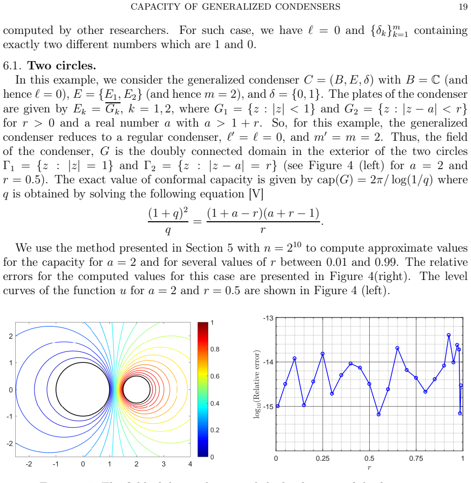
Compute the capacity of the two-circle condenser in Section 6.1 with increasing $n$ and compare it with the exact value $2\pi/\log(1/q)$: if the relative error does not converge toward machine precision, the derived equations are not producing the constants $a_k$. A sharper test targets the branch-cut settings of Lemma 3.9: move the auxiliary points across different branch choices and check whether the computed capacity changes.

Watch

Extended reading notes

Core claim

The central claim is that for a generalized condenser $C=(B,E,\delta)$ whose plates are bordered by piecewise smooth Jordan curves or rectilinear slits, the capacity $\operatorname{cap}(C)$ is obtained numerically from the formula $\operatorname{cap}(C)=2\pi\sum_{k=1}^m \delta_k a_k$, where the constants $a_k$ are found by solving the generalized Neumann kernel equations $(I-N)\mu_k=-M\gamma_k$ and then one linear system whose entries come from the piecewise-constant functions $h_k$. The argument reduces the mixed Dirichlet-Neumann problem for the potential to a Riemann-Hilbert problem for an auxiliary analytic function, uses the unique solvability of the generalized Neumann kernel equation to construct basis functions, and proves that the derived linear systems are non-singular. On this basis the same algorithm computes the potential $u$ in the field by Cauchy's integral formula and the harmonic measure for multiply connected domains.

Load-bearing premise

The method stands on the unique-solvability theory of the generalized Neumann kernel equations and of the derived linear systems: if those systems can fail to have exactly one solution for the piecewise-constant data used here, the constants $a_k$, and with them the capacity formula, would not be determined by the numerical solution.

Editorial extensions

If this is right

Capacities of generalized condensers with thousands of boundary components, such as Cantor-dust and Sierpinski-carpet approximations, become computable in seconds to minutes.
The same solver computes harmonic measure in multiply connected domains, including piecewise-smooth boundary components, by taking the level vector $\delta$ to be 1 on one boundary component and 0 on the others.
Rectilinear-slit condensers are covered by first mapping the slit domain conformally to a smooth-bordered domain, since capacity is conformally invariant, so the scope extends beyond Jordan-curve boundaries.
The cost estimate $O(m'(m+\ell)n\log n)$ for the integral-equation step, with only a small linear system afterwards, makes large many-plate problems feasible on a laptop.

Reading between the lines

Editorial extensions of the paper, not claims the author makes directly.

Because the capacity formula is linear in the potential levels $\delta_k$, one set of constants $a_k$ can be reused for many level assignments; the paper does not advertise this, but it follows directly from (2.12).
The separation into an integral-equation stage and a tiny linear stage suggests the constants $a_k$, which are essentially boundary flux integrals, could serve as building blocks for other conformal invariants that are Dirichlet integrals over the same field.
For slit plates the accuracy of the final capacity is inherited from the separately computed conformal map; a direct integral formulation on slit boundaries would remove that intermediate step, and the boundary conditions derived here give a starting point for such a formulation.
The uniqueness lemma for piecewise-constant right-hand sides, if it extends to other coefficient functions $A$, could yield numerical methods for a wider class of mixed boundary-value problems than the constant-level case treated in this paper.

Share X Bluesky LinkedIn Reddit HN

Signed reviews

No signed human review yet.

Editorial analysis

A structured set of objections, weighed in public.

Desk editor's note, referee report, and a circularity audit.

Desk Editor's Note

read the letter

Here's my read of Nasser–Vuorinen. The headline is good news: they give the first numerical method for capacity of generalized condensers—multiple plates with different potential levels, mixed Dirichlet/Neumann boundaries, slit geometries—by reducing the problem to a Riemann–Hilbert problem and solving it with the generalized Neumann kernel. That isn't just a repackaging: the linear systems (4.11)/(4.24) that determine the flux constants are new, and they make the capacity calculation (2.12) direct. The code is public, and the validation on regular condensers (two circles, [BSV] tables, Cantor dust) matches exact or published values to 6–12 digits. That is real evidence the machinery works.

The theoretical chain from (2.6) to (2.12) is standard and, as far as I can tell, correct. The soft spots are real but not load-bearing. Lemma 4.7, which guarantees that the piecewise-constant right-hand side in (4.11) is uniquely determined, gets a one-paragraph proof that leans on an external uniqueness theorem from [N3, WN] stated in weaker form. The stress-test worry is whether that theorem covers arbitrary piecewise-constant γ and the branch-cut-dependent γ_k. I think it does: piecewise constants on disjoint boundary curves are Hölder continuous, and Lemma 3.9 exists precisely to make the γ_k single-valued. But the paper should say what theorem is being used and in what generality. Theorem 4.22 is explicitly unproved ('same argument'), which is fine if true but needs checking. The other soft spot is that Sections 7–8 (true generalized condensers) have no independent benchmarks, so the error is only demonstrated indirectly; a referee should ask for at least one check against a known or asymptotic case. Minor: Table 4 has a duplicated δ2 value (0.15 appears twice, presumably 0.75).

This is a paper for computational complex analysis and potential theory. It deserves a serious referee; the right recommendation is likely 'major revision' with the requested expansions, not rejection. I'd take it to the reading group.

Referee Report

2 major / 5 minor

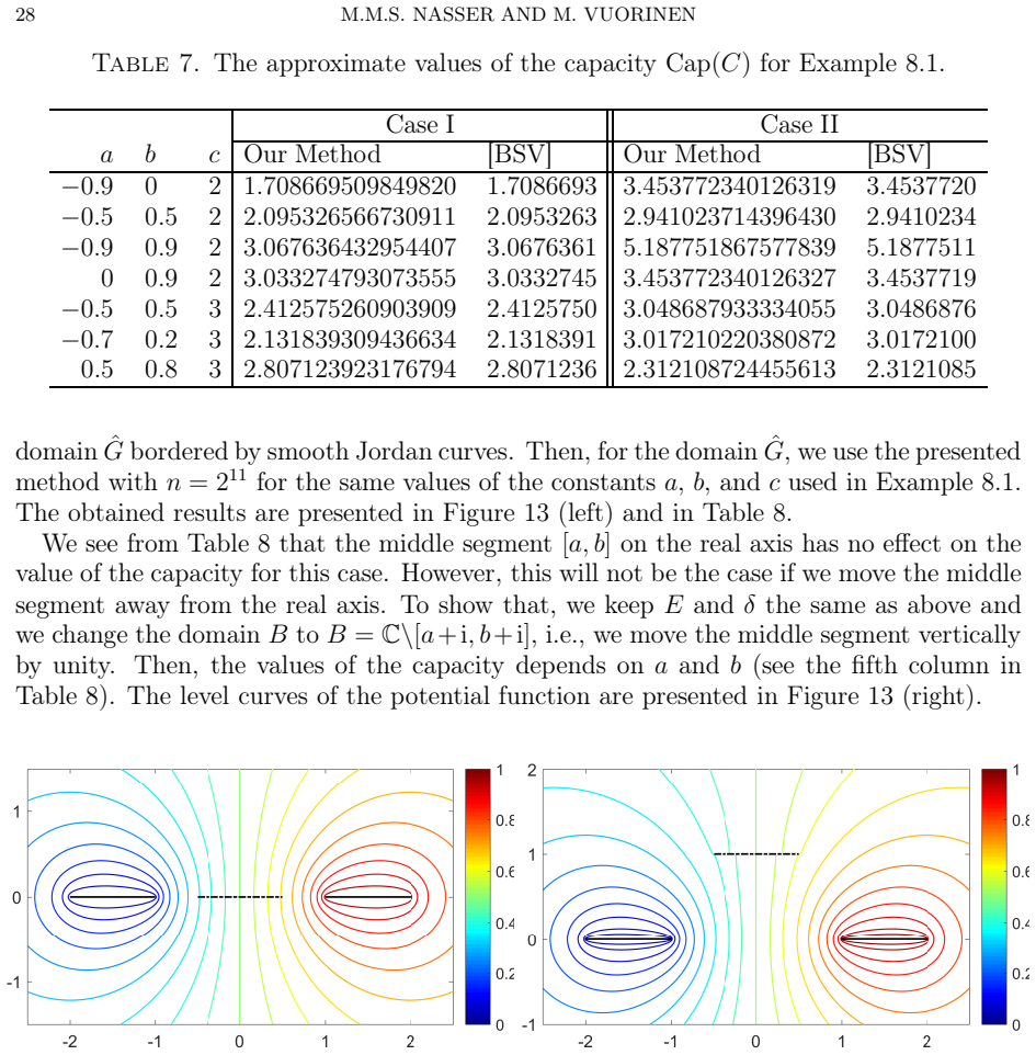
Summary. This paper presents a boundary integral method for computing the conformal capacity of generalized condensers (B, E, δ) in the complex plane. The plates E_k are closures of simply connected domains bounded by piecewise smooth Jordan curves; rectilinear-slit plates are handled via auxiliary conformal mappings. The mixed Dirichlet–Neumann problem for the potential u is reduced to a Riemann–Hilbert problem, and the generalized Neumann kernel is used to obtain a representation of the boundary values of the auxiliary analytic function in terms of flux constants a_k. The main theoretical results, Theorems 4.9 and 4.22, assert that the a_k satisfy a small dense linear system (4.11) or (4.24); the capacity is then cap(C) = 2π Σ δ_k a_k. The paper includes a MATLAB implementation, numerical validation against exact two-circle capacities and published [BSV] tables, and examples with Cantor dust, Sierpinski carpets, slit condensers, and harmonic measure computations.

Significance. If the theoretical framework is correct, this is the first numerical method for capacities of generalized condensers with piecewise smooth boundaries, and it also computes harmonic measure in multiply connected domains. The method has near-linear complexity in the discretization size, is validated to 6–12 digits against independent benchmarks, and is demonstrated on domains with thousands of boundary components. The full MATLAB code is provided, making the computational claims reproducible. The paper's practical contribution is substantial; the main caveat is the need for a more complete statement and proof of the uniqueness result on which the linear systems rely.

major comments (2)

[Section 4, Lemma 4.7] The proof of Lemma 4.7 is load-bearing for Theorems 4.9 and 4.22, but as written it is not self-contained. It invokes 'a unique piecewise constant real-valued function h' making Re[A f] = γ + h uniquely solvable, whereas the only stated result of this type, Theorem 4.3, is proved or cited only for the particular functions γ_k defined in (3.10). Lemma 4.7 requires the external theorem from [N3,WN] to hold for every piecewise constant, indeed every Hölder continuous, right-hand side γ, together with uniqueness of the pair (f,h) under the normalization f(∞)=0 for unbounded G (and the corresponding normalization for bounded G). Please state the general theorem explicitly and verify that the branch-cut/winding-number hypotheses are satisfied under Lemma 3.9; this is what justifies the conclusion h = −γ and hence the invertibility of the linear systems (4.11) and (4.24).
[Section 4, Theorem 4.22] The proof of Theorem 4.22 is omitted with the justification 'the theorem can be proved by the same argument as in the proof of Theorem 4.9.' This is not a routine omission because the Case II linear system (4.24) differs structurally from (4.11): there is no explicit Σ a_k = 0 row, a_m is recovered afterwards from (2.10), and the role of the exterior plate E_m changes the normalization argument in the bounded-G case. The nonsingularity of (4.24) and the derivation of the homogeneous solution are therefore not immediate corollaries of the proof of Theorem 4.9. Please provide a complete proof or a detailed set of modifications.

minor comments (5)

[Section 4] The sentence 'The integral equation (4.5) been used for computing...' should read 'has been used for computing...'.
[Table 4] The fifth row lists δ2 = 0.15; from the monotone sequence 0.15, 0.30, 0.45, 0.60, 0.90 this appears to be a typo, probably 0.75.
[Algorithm 4.26, step 2] Step 2 ends with 'Γ_j for j = m + 1, m + 2, ..., m'; the upper limit should be m + ℓ.
[Section 3, proof of Lemma 3.9] The proof contains an algebraic identity that is valid only because Σ a_k = 0; a remark at the point where Re[e^{-iθ} log(η−α)] Σ a_k is introduced would improve readability.
[References] The reference [Ku1] is listed but not cited in the text; either cite it or remove it.

Circularity Check

0 steps flagged · score 0.0 of 10

No significant circularity: capacity is computed from BVP flux constants and checked against independent benchmarks.

full rationale

Section 4.3 obtains cap(C) from (2.12), a Green's-formula identity cap(C)=2πΣδ_k a_k with a_k the flux integrals (2.5)/(2.8). The a_k are not fitted to capacity; they are the solution of the linear systems (4.11)/(4.24) assembled from the µ_k, h_k computed by solving integral equation (4.5). The derivation of the linear systems (Theorem 4.9) uses Lemma 4.7 and the cited generalized Neumann kernel theory [N3, WN]; that theory is external mathematical tooling (solvability of Riemann-Hilbert problems), not the target capacity result, and its assumptions do not include the values being computed. Numerical checks are independent: exact two-circle capacity (Section 6.1), published [BSV] tables (Sections 6.2 and 8.1), and exact annulus harmonic measure (Section 9.2). Slit-plate examples use conformal mapping from [NG] to smooth domains, but capacity invariance under conformal maps is a standard theorem and the mapping is auxiliary. The terse proof of Lemma 4.7 extrapolates Theorem 4.3 from the specific γ_k to arbitrary piecewise-constant γ; this is a possible rigor gap in the cited solvability theory, not a circular definition or a fitted-input prediction. No equation here reduces to its own input by construction.

Assumptions & free parameters 2 free parameters · 5 assumptions · 0 invented entities

The central derivation inherits the existence and uniqueness theory of the mixed BVP, the logarithmic representation of harmonic functions, and the generalized Neumann kernel solvability from prior literature. No new physical entities are postulated. The hand-chosen numbers are algorithmic (auxiliary points, n, tolerances) and do not encode target capacities.

free parameters (2)

Auxiliary points alpha_k (k=1..m') and alpha = Arbitrary; placed inside bounded complementary domains
Chosen by hand in (2.6)/(3.10) to define the logarithm branches. The capacity (2.12) is theoretically independent of these locations, so they are not fitted to target data.
Discretization size n and iterative solver tolerances = n between 2^8 and 2^11; GMRES tol 1e-14; FMM tol 0.5e-15
Set by the authors for accuracy. Convergence in n is demonstrated in Example 7.2 and by benchmark agreements, but no certified a posteriori error bound is supplied.

assumptions (5)

standard math The mixed Dirichlet-Neumann boundary value problem (2.3) has a unique solution u.
Used in Section 2 to justify the potential representation and in Theorem 4.9 to identify constant solutions; cited to [IS].
standard math The harmonic function u is the real part of an analytic F of the form F(z) = g(z) - sum a_k log(z-alpha_k) with single-valued g and real constants a_k.
Equation (2.6), from Mikhlin Section 31; it is the foundation of the Riemann-Hilbert reduction.
standard math For the functions gamma_k in (3.10), the integral equation (I-N)mu_k = -M gamma_k is uniquely solvable and a unique piecewise constant h_k exists such that Re[A f_k] = gamma_k + h_k.
Theorem 4.3 cited to [N3,WN]; Lemma 4.7 and Theorems 4.9/4.22 depend on this external result.
standard math The Dirichlet integral is conformally invariant, so a conformally equivalent smooth domain has the same capacity.
Used in Section 8 to justify replacing slit boundaries by smooth curves via the [NG] mapping method.
domain assumption Trapezoidal rule with equidistant nodes converges exponentially for smooth boundaries, and Kress graded meshes restore convergence at corners.
Section 5 selects quadrature; the numerical success of the tests is empirical evidence for this assumption.

how reviews work

0 comments

Cite this review

Pith. "Pith review of Numerical computation of the capacity of generalized condensers." pith.science (2026). https://pith.science/paper/7GOJNMVO

@misc{pith2026190803866,
  author       = {Pith},
  title        = {Pith review of: Numerical computation of the capacity of generalized condensers},
  year         = {2026},
  howpublished = {\url{https://pith.science/paper/7GOJNMVO}},
  note         = {Machine review of arXiv:1908.03866}
}

read the original abstract

We present a boundary integral method for numerical computation of the capacity of generalized condensers. The presented method applies to a wide variety of generalized condenser geometry including the cases when the plates of the generalized condenser are bordered by piecewise smooth Jordan curves or are rectilinear slits. The presented method is used also to compute the harmonic measure in multiply connected domains.

Figures

Figures reproduced from arXiv: 1908.03866 by the authors.

**Figure 2.** An example of a bounded multiply connected domain G for m = 3 and ℓ = 3 for Case I (both G and B are bounded) [PITH_FULL_IMAGE:figures/full_fig_p010_2.png] view at source ↗

**Figure 3.** An example of a bounded field of the condenser G for m = 3 and ℓ = 3 for case II (m′ = m − 1, ℓ ′ = ℓ). Theorem 4.22. For each k = 1, 2, . . . , m − 1, let the function γk be defined by (3.10), let µk be the unique solution of the integral equation (4.5), and let the piecewise constant function hk = (h1,k, h2,k, . . . , hm+ℓ,k) be given by (4.6). Then, the boundary values of the function f in (3.15) are given by (4.… view at source ↗

Figures from the paper (13 more)

**Figure 4.** Figure 4: The field of the condenser and the level curves of the function u for Example 6.1 (left) and the relative errors in the computed values (right). 6.2. Square with two triangles. In this example, we consider the generalized condenser C = (B, E, δ) with B = C, E = {E1, E2…

**Figure 5.** Figure 5: The field of the condenser and the level curves of the function u for the condenser in Example 6.2 [PITH_FULL_IMAGE:figures/full_fig_p020_5.png]

**Figure 6.** Figure 6: The level curves of the function u for the condenser in Example 6.3 for k = 1 (left) and k = 2 (right) [PITH_FULL_IMAGE:figures/full_fig_p022_6.png]

**Figure 7.** Figure 7: The level curves of the function u for the condenser in Example 6.4 for k = 1 (left) and k = 2 (right). |z − 2| = r}, Γ2 = {z : |z − 2| = r}, L1,2 = {z : |z ∓ 2i| = 0.9}, L3 = {z : |z + 2| = 0.9}, and interior to the circles L4 = {z : |z| = 3} (see [PITH_FULL_IMAGE:f…

**Figure 8.** Figure 8: The field of the condenser and the level curves of the function u for B = BI (left) and B = BII (center); and the approximate values of the capacity for δ2 = 1 (right). 7.2. Five circles. In this example, we consider the generalized condenser C = (B, E, δ) with B = C, …

**Figure 9.** Figure 9: The field of the condenser and the level curves of the function u for the condenser in Example 7.2. (see [PITH_FULL_IMAGE:figures/full_fig_p025_9.png]

**Figure 10.** Figure 10: The level curves of the function u for the condenser in Example 7.3 for k = 2 (left) and k = 3 (right). 8. Condensers with slit plates The method presented above can be used to compute the capacity of only condensers bordered by smooth or piecewise smooth boundaries.…

**Figure 11.** Figure 11: The domains G (left) and Gˆ (right) for the condenser in Example 8.1. Since the Dirichlet integral is conformally invariant, the capacity for the new domain Gˆ is the same as the capacity for the original domain G. For the new domain Gˆ, we use the presented method wi…

**Figure 12.** Figure 12: The level curves of the function u for the condenser in Example 8.1 for Case I (left) and Case II (right). 8.2. Three slits: generalized condenser. In this example, we consider the generalized condenser C = (B, E, δ) with B = C\[a, b], E = {E1, E2} where E1 = [−c, −1…

**Figure 13.** Figure 13: The level curves of the function u for the condenser in Example 8.2 for B = C\[a, b] (left) and B = C\[a + i, b + i] (right). 8.3. Cantor set. In Example 6.3, we consider the Cantor dust which a generalization of the classical Cantor middle third set to dimension two…

**Figure 14.** Figure 14: for k = 2 (left) and k = 3 (right)). We consider the generalized condensers Ck = (B, E, δ) with B = C and E = {E1, E2, . . . , E2 k }. For the levels of the potential function δ = {δj} 4 k j=1, we assume δj = 0 for half of the plates (the plates on the left of the lin…

**Figure 15.** Figure 15: The level curves of the absolute error in the computed values of the harmonic measures ωG,Γ1 (z) (left) and ωG,Γ2 (z) (right) for Example 9.2. 9.3. Two disks and two polygons. We consider the multiply connected domain G of connectivity 4 in the exterior of the curves …

**Figure 16.** Figure 16: The level curves of the computed harmonic measures ωG,Γ1 (z) (top, left), ωG,Γ2 (z) (top, right), ωG,Γ3 (z) (bottom, left), and ωG,Γ4 (z) (bottom, right) for Example 9.3. [AT] K.E. Atkinson, The Numerical Solution of Integral Equations of the Second Kind. Cambridge U…

Discussion (0). Continue with ORCID to comment.

Reference graph

Works this paper leans on

45 extracted references · 45 canonical work pages

[1]

Ahlfors, Conformal invariants

L.V. Ahlfors, Conformal invariants. McGraw-Hill, New York, 1973

work page 1973
[2]

Al-Hatemi, A.H.M

S.A.A. Al-Hatemi, A.H.M. Murid and M.M.S. Nasser , A boundary integral equation with the generalized Neumann kernel for a mixed boundary value problem in unbounded multiply connected regions. Bound. Value Probl. 2013 (2013), Article No. 54

work page 2013
[3]

G. D. Anderson, M. K. Vamanamurthy, and M. Vuorinen, Conformal invariants, inequalities and quasiconformal maps. John Wiley, 1997

work page 1997
[4]

Aoyama, T

N. Aoyama, T. Sakajo and H. Tanaka,

work page
[5]

Atkinson , The Numerical Solution of Integral Equations of the Second Kind

K.E. Atkinson , The Numerical Solution of Integral Equations of the Second Kind. Cambridge University Press, 1997

work page 1997
[6]

Bezrodnykh, A

S. Bezrodnykh, A. Bogatyrev, S. Goreinov, O. Grigoriev, H. Hakula, and M. Vuorinen : On capacity computation for symmetric polygonal condensers. J. Comput. Appl. Math. 361 (2019), 271--282

work page 2019
[7]

Betsakos, K

D. Betsakos, K. Samuelsson, and M. Vuorinen, The computation of capacity of planar condensers. Publ. Inst. Math. (Beograd) (N.S.) 75(89) (2004), 233--252

work page 2004
[8]

Crowdy and J

D. Crowdy and J. Marshall , Green's functions for Laplace equation in multiply connected domains. IMA J. Appl. Math. 72 (2007), 278--301

work page 2007

Show all 45 references

[9]

Driscoll and L.N

T.A. Driscoll and L.N. Trefethen, Schwarz-Christoffel mapping. Cambridge Monographs on Applied and Computational Mathematics, 8. Cambridge University Press, Cambridge, 2002. xvi+132 pp

2002
[10]

DeLillo, A.R

T.K. DeLillo, A.R. Elcrat and E.H. Kropf , Calculation of resistances for multiply connected domains using Schwarz-Christoffel transformations. Comput. Methods Funct. Theory 11 (2011), 725--745

2011
[11]

V. N. Dubinin, Condenser Capacities and Symmetrization in Geometric Function Theory, Birkh\"auser, 2014

2014
[12]

V. N. Dubinin , Capacities of condensers, generalizations of Gr\"otzsch lemmas, and symmetrization. Journal of Mathematical Sciences 143 (2007), 3053--3068

2007
[13]

V. N. Dubinin and N. V. Eyrikh , Applications of Generalized Condensers to Analytic Function Theory. Journal of Mathematical Sciences 133 (2006), 1634--1647

2006
[14]

V. N. Dubinin and D. B. Karp , Generalized condensers and distortion theorems for conformal mappings of planar domains. Contemporary Mathematics 424 (2007), 33--52

2007
[15]

V. N. Dubinin and D. Karp , Capacities of certain plane condensers and sets under simple geometric transformations. Complex Var. Elliptic Equ. 53(6) (2008), 607--622

2008
[16]

Gakhov, Boundary Value Problems, Pergamon Press, Oxford, 1966

F.D. Gakhov, Boundary Value Problems, Pergamon Press, Oxford, 1966

1966
[17]

J. B. Garnett and D. E. Marshall, Harmonic measure. Reprint of the 2005 original. New Mathematical Monographs, 2. Cambridge University Press, Cambridge, 2008. xvi+571 pp

2005
[18]

Greengard and Z

L. Greengard and Z. Gimbutas , FMMLIB2D: A MATLAB toolbox for fast multipole method in two dimensions. Version 1.2, http://www.cims.nyu.edu/cmcl/fmm2dlib/fmm2dlib.html. Accessed 1 Jan 2018

2018
[19]

Haas and H

R. Haas and H. Brauchli , Fast solver for plane potential problems with mixed boundary conditions. Comput. Methods Appl. Mech. Engrg. 89 (1991), 543--556

1991
[20]

Hakula, A

H. Hakula, A. Rasila and M. Vuorinen , On moduli of rings and quadrilaterals: algorithms and experiments. SIAM J. Sci. Comput. 33 (2011), 279--302

2011
[21]

Hakula, A

H. Hakula, A. Rasila and M. Vuorinen , Computation of exterior moduli of quadrilaterals. Electron. Trans. Numer. Anal. 40 (2013), 436--451

2013
[22]

P. N. Ivanshin and E. A. Shirokova , The solution of a mixed boundary value problem for the Laplace equation in a multiply connected domain. Probl. Anal. Issues Anal. 8 (26) (2019), 51--66

2019
[23]

Krantz , Geometric Function Theory: Explorations in Complex Analysis

S.G. Krantz , Geometric Function Theory: Explorations in Complex Analysis. Birkh\"auser, Boston, 2006

2006
[24]

Kress , A Nystr\"om method for boundary integral equations in domains with corners

R. Kress , A Nystr\"om method for boundary integral equations in domains with corners. Numer. Math. 58(2) (1990), 145--161

1990
[25]

K\"uhnau , Boundary Effects for an Electrostatic Condenser

R. K\"uhnau , Boundary Effects for an Electrostatic Condenser. Journal of Mathematical Sciences, 105 (2001), 2210--2219

2001
[26]

uhnau,\, The conformal module of quadrilaterals and of rings, In: Handbook of Complex Analysis: Geometric Function Theory , (ed. by R. K\

R. K\"uhnau,\, The conformal module of quadrilaterals and of rings, In: Handbook of Complex Analysis: Geometric Function Theory , (ed. by R. K\"uhnau) Vol. 2, North Holland/Elsevier, Amsterdam, 99--129, 2005

2005
[27]

Lehto and K.I

O. Lehto and K.I. Virtanen,\,
[28]

Liesen, O

J. Liesen, O. S\'ete and M.M.S. Nasser , Fast and accurate computation of the logarithmic capacity of compact sets. Comput. Methods Funct. Theory 17 (2017), 689--713

2017
[29]

Mikhlin, Integral Equations and Their Applications to Certain Problems in Mechanics, Mathematical Physics and Technology

S.G. Mikhlin, Integral Equations and Their Applications to Certain Problems in Mechanics, Mathematical Physics and Technology. 2nd rev ed. Pergamon Press, Oxford, 1964

1964
[30]

Muskhelishvili, Singular Integral Equations, Noordhoff, Groningen, 1953

N.I. Muskhelishvili, Singular Integral Equations, Noordhoff, Groningen, 1953

1953
[31]

Nasser , Numerical conformal mapping via a boundary integral equation with the generalized Neumann kernel

M.M.S. Nasser , Numerical conformal mapping via a boundary integral equation with the generalized Neumann kernel. SIAM J. Sci. Comput. 31 (2009), 1695--1715

2009
[32]

Nasser , Numerical conformal mapping of multiply connected regions onto the second, third and fourth categories of Koebe canonical slit domains

M.M.S. Nasser , Numerical conformal mapping of multiply connected regions onto the second, third and fourth categories of Koebe canonical slit domains. J. Math. Anal. Appl. 382 (2011), 47--56

2011
[33]

Nasser , Fast solution of boundary integral equations with the generalized Neumann kernel

M.M.S. Nasser , Fast solution of boundary integral equations with the generalized Neumann kernel. Electron. Trans. Numer. Anal. 44 (2015), 189--229

2015
[34]

Nasser, J

M.M.S. Nasser, J. Liesen and O. S\'ete , Numerical computation of the conformal map onto lemniscatic domains. Comput. Methods Funct. Theory 16 (2016), 609--635

2016
[35]

Nasser, A.H.M

M.M.S. Nasser, A.H.M. Murid and S.A.A. Al-Hatemi , A boundary integral equation with the generalized Neumann kernel for a certain class of mixed boundary value problem. J. Appl. Math. 2012 (2012), Article ID 254123, 17 pages

2012
[36]

Nasser and C.C

M.M.S. Nasser and C.C. Green , A fast numerical method for ideal fluid flow in domains with multiple stirrers. Nonlinearity 31 (2018), 815--837

2018
[37]

Papamichael and N

N. Papamichael and N. Stylianopoulos , Numerical conformal mapping: Domain decomposition and the mapping of quadrilaterals. World Scientific; 2010

2010
[38]

Ransford , Computation of logarithmic capacity

T. Ransford , Computation of logarithmic capacity. Comput. Methods Funct. Theory 10(2) (2010), 555–578

2010
[39]

Ransford and J

T. Ransford and J. Rostand , Computation of capacity. Math.Comput.76(259) (2007), 1499--1520

2007
[40]

Trefethen and J

L.N. Trefethen and J. A. C. Weideman , The exponentially convergent trapezoidal rule. SIAM Review 56 (2014), 385--458

2014
[41]

Tsuji , Potential Theory in Modern Function Theory

M. Tsuji , Potential Theory in Modern Function Theory. Chelsea Publ. Co., New York, 1975

1975
[42]

Vasil ' ev , Moduli of Families of Curves for Conformal and Quasiconformal Mappings

A. Vasil ' ev , Moduli of Families of Curves for Conformal and Quasiconformal Mappings. Springer-Verlag, Berlin, 2002

2002
[43]

Vuorinen , Conformal geometry and quasiregular mappings

M. Vuorinen , Conformal geometry and quasiregular mappings. Lecture Notes in Mathematics, 1319. Springer-Verlag, Berlin, 1988

1988
[44]

Vuorinen : Conformal invariants and quasiregular mappings

M. Vuorinen : Conformal invariants and quasiregular mappings. - J. Anal. Math. 45 (1985), 69--115

1985
[45]

Wegmann and M.M.S

R. Wegmann and M.M.S. Nasser , The Riemann-Hilbert problem and the generalized Neumann kernel on multiply connected regions. J. Comput. Appl. Math. 214 (2008), 36--57

2008

Pith tools

Reviewed August 14, 2026 · model on record in the stance chip above.

[1] [1]

Ahlfors, Conformal invariants

L.V. Ahlfors, Conformal invariants. McGraw-Hill, New York, 1973

work page 1973

[2] [2]

Al-Hatemi, A.H.M

S.A.A. Al-Hatemi, A.H.M. Murid and M.M.S. Nasser , A boundary integral equation with the generalized Neumann kernel for a mixed boundary value problem in unbounded multiply connected regions. Bound. Value Probl. 2013 (2013), Article No. 54

work page 2013

[3] [3]

G. D. Anderson, M. K. Vamanamurthy, and M. Vuorinen, Conformal invariants, inequalities and quasiconformal maps. John Wiley, 1997

work page 1997

[4] [4]

Aoyama, T

N. Aoyama, T. Sakajo and H. Tanaka,

work page

[5] [5]

Atkinson , The Numerical Solution of Integral Equations of the Second Kind

K.E. Atkinson , The Numerical Solution of Integral Equations of the Second Kind. Cambridge University Press, 1997

work page 1997

[6] [6]

Bezrodnykh, A

S. Bezrodnykh, A. Bogatyrev, S. Goreinov, O. Grigoriev, H. Hakula, and M. Vuorinen : On capacity computation for symmetric polygonal condensers. J. Comput. Appl. Math. 361 (2019), 271--282

work page 2019

[7] [7]

Betsakos, K

D. Betsakos, K. Samuelsson, and M. Vuorinen, The computation of capacity of planar condensers. Publ. Inst. Math. (Beograd) (N.S.) 75(89) (2004), 233--252

work page 2004

[8] [8]

Crowdy and J

D. Crowdy and J. Marshall , Green's functions for Laplace equation in multiply connected domains. IMA J. Appl. Math. 72 (2007), 278--301

work page 2007