REVIEW 4 major objections 4 minor 20 references
Maximizing Ink in Partial Edge Drawings of k-plane Graphs
T0 review · 4 major / 4 minor · reviewed 2026-08-14 · deepseek-v4-flash
Pith's one-line read This paper proves exact ink-maximization for partial edge drawings is NP-hard once crossings per edge reach three (SPED) or four (PED), and gives polynomial/XP algorithms when the edge-intersection graph is a tree or has bounded treewidth.
desk verdict Sound treewidth algorithms plus a credible but incomplete MaxPED hardness proof; Appendix A needs a formal epsilon argument and corrected ink arithmetic before the complexity claim is citable. read the letter →
The pith
A machine-rendered reading of the paper's core claim, the machinery that carries it, and where it could break.
The reading
What carries the argument
The central object is the edge intersection graph C of the drawing: a vertex for every drawn edge and an edge for every crossing. Since the drawing is k-plane, C has maximum degree k. The finite-state insight is that a segment s(u) with delta_u crossings has only delta_u + 1 relevant stub-length choices (the lengths cut off at successive intersection points, plus the full segment). The tree algorithm stores W_i(u), the best ink in the subtree of C when s(u) is drawn with the i-th stub length, and separates child contributions into short(v) (choices that do not constrain the parent) and long(v) (those that do). The bounded-treewidth algorithm stores W(t,S) for each node t of a nice tree decomposition: S is a valid choice of stubs on the bag X_t, and W(t,S) is the best ink in V_t consistent with S, combined through leaf, introduce, forget, and join recurrences. All of the work, both hardness and tractability, flows from the fact that only these finitely many stub lengths per edge matter.
What would settle it
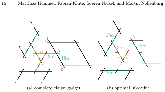
Set alpha = 2 beta in the Theorem 2 gadgets and exhaustively enumerate all stub/gap placements for one variable gadget and one clause gadget, computing the true maximum ink by brute force; the reduction requires the variable gadget's per-segment maximum to be alpha + beta, the clause gadget's maximum to be 221 alpha + 30 beta, and any placement that gains 3 alpha by drawing a connecting section to lose at least 9 alpha in the attached weight component, so any configuration exceeding these totals would break the threshold L.
Extended reading notes
Core claim
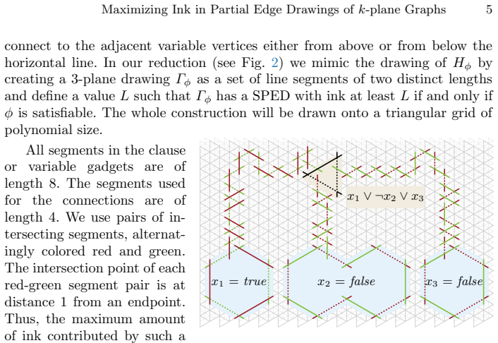
The paper establishes two complexity thresholds. For symmetric partial edge drawings, deciding whether a given straight-line drawing admits a solution with ink at least L is NP-hard already for 3-plane input drawings, where no edge crosses more than three others; the reduction uses planar 3-SAT, with variable gadgets that have exactly two maximum-ink states (encoding true/false) and clause gadgets that reach their maximum ink only when at least one literal is satisfied. For general (asymmetric) partial edge drawings, the same decision problem is NP-hard for 4-plane input drawings; because the stubs are independent, the construction works with an arbitrarily small erased gap per edge and uses the position of that gap to encode truth values, with a clause gadget whose weight components make it too expensive to draw more than one full triangle segment. Complementing these hardness results, the paper gives exact dynamic programs for both problems when the edge intersection graph is a tree, with running times O(mk + m log m) and O($mk^{2}$ + m log m), and XP algorithms when that graph has treewidth at most omega, with running times exponential only in omega. Corollary: neither problem is fixed-parameter tractable when parameterized by the crossing number k alone.
Load-bearing premise
The hardness proofs assume the exact ink values assigned to each gadget are correct and that the tiny erased gap in the MaxPED construction can be made uniformly small enough that no other configuration overturns the claimed optimum; if that accounting fails, the equivalence between high-ink drawings and satisfying truth assignments collapses.
Editorial extensions
If this is right
- MaxSPED has no polynomial algorithm for 3-plane drawings unless P = NP; together with the known polynomial algorithm for 2-plane drawings, this puts the tractability threshold exactly at k = 2 for symmetric stubs.
- MaxPED is NP-hard for 4-plane drawings; the 3-plane case remains open, and Corollary 1 rules out fixed-parameter tractability by k alone for both problems.
- If the edge intersection graph is a tree, maximum-ink SPEDs and PEDs can be computed exactly in O(mk + m log m) and O(mk^2 + m log m) time, respectively.
- If the intersection graph has treewidth at most omega, both problems are solvable in time exponential only in omega: O(m(k+1)^{omega+2} omega^2 + m log m) for MaxSPED and O(m(k+1)^{omega+3} omega^2 + m log m) for MaxPED.
- The implemented treewidth algorithm preserves, on the tested layouts, roughly 84-90% of the ink for SPEDs and 97-99% for PEDs, showing that the exact optimum leaves only moderate erasure on those instances.
Reading between the lines
- By extension, the same finite stub-choice DP should solve fixed-ratio asymmetric homogeneous PEDs on trees and bounded-treewidth crossing graphs; the paper names this as an expected but unresolved direction.
- Because the MaxPED hardness proof lets the erased gap shrink to zero, a natural stress test is to recompute the reduction with one fixed positive gap size; if no single epsilon works for every gadget, the hardness threshold could depend on the gap, not just on k.
- The dichotomy suggests a practical heuristic: even drawings with many crossings can be solved exactly whenever the crossing graph is near-forest, so an exact solver should measure treewidth first and fall back to heuristics only when treewidth is large.
Signed reviews
Editorial analysis
A structured set of objections, weighed in public.
Referee Report
Summary. The paper studies the ink-maximization problem for partial edge drawings (PEDs) and symmetric partial edge drawings (SPEDs) of k-plane straight-line drawings. The main theoretical contributions are: (1) NP-hardness of MaxSPED for 3-plane input drawings (Theorem 1), (2) NP-hardness of MaxPED for 4-plane input drawings (Theorem 2), (3) polynomial-time algorithms for both problems when the edge intersection graph of the drawing is a tree (Theorem 3 and Corollary 2), and (4) XP algorithms parameterized by the treewidth of the intersection graph (Theorem 4 and Corollary 3). The paper also reports a proof-of-concept implementation and experiments on spring and circular layouts. The algorithmic parts are clearly structured and the dynamic-programming recurrences appear correct. The hardness proof for MaxPED, however, is not complete as written: it relies on an unformalized ε→0 limit and contains internal inconsistencies in the ink accounting of the gadgets.
Significance. If the hardness results are established, they settle a conjecture of Bruckdorfer and close the complexity gap for MaxPED on k-plane drawings for k≥4, while also strengthening the known hardness of MaxSPED to 3-plane inputs. The treewidth-based algorithms are a genuine positive contribution: they give a clean XP parameterization and, for the forest case, simple polynomial-time dynamic programs that are also implemented and experimentally evaluated. The DP recurrences (Section 4) and the running-time analyses are presented in a way that is easy to verify, and the implementation is a useful proof of concept. The main weakness is the MaxPED NP-hardness proof in Appendix A, which is load-bearing for the paper's central claim and currently contains gaps that prevent the reduction from being considered rigorous.
major comments (4)
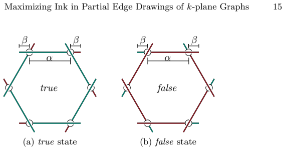
- [Appendix A, first paragraph] The proof of Theorem 2 assumes l(s)+r(s)=1 for every segment, i.e., it works with zero-width gaps, and encodes truth states via which stub is longer. A genuine PED requires a positive erased gap, so the actual ink per segment is |s|-ε. The paper never proves that a single ε>0 works uniformly across all variable, wire, and clause gadgets, and the threshold L is computed without any ε. Since the set of valid configurations can change in the limit ε→0 (for example, stubs that merely touch at a crossing are treated as non-crossing), the equivalence I(D)≥L iff satisfiable is not established by the argument as written.
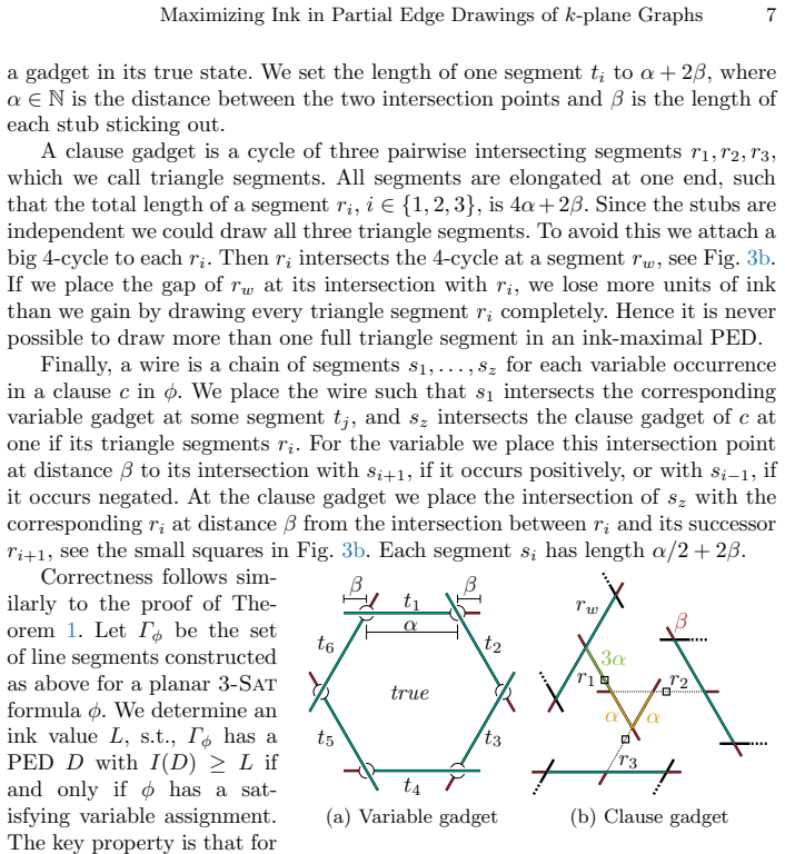
- [Appendix A, variable gadget] The ink accounting for the variable gadget is internally inconsistent. The segment length is defined as |s_i|=α+2β, and it is stated that G(x) admits a PED with I(G(x))=Σ|s_i|, but the proof then asserts I(G(x))=|G(x)|·(α+β). If |G(x)| denotes the number of segments, this is off by β per segment; if it denotes something else, that quantity is never defined. Since L is defined as the sum of gadget maxima, this discrepancy propagates into the wire-loss analysis and the correctness argument.
- [Appendix A, clause gadget] The claimed maximum ink value of the clause gadget, I(G(c)) = 3·(72α+8β)+5α+6β = 221α+30β, is asserted without a derivation of the 5α+6β internal contribution. The internal component consists of three segments of total length 12α+6β, so the claimed loss of 7α from the internal component is not reconciled with the geometry. In particular, the argument that placing the gap of an internal segment anywhere other than at its weight-component intersection loses 'at least 9α units of ink' is not substantiated, and the text does not explain why the configuration achieving 5α+6β is valid while alternative configurations are not. Because the threshold L and the reduction's iff depend on this value, the proof is incomplete.
- [Section 3.1, Theorem 1] The converse direction of the MaxSPED reduction is dismissed with 'it is straight-forward to verify that the corresponding truth assignment satisfies φ'. Given the complexity of the variable and clause gadgets and the wire connections, the proof needs an explicit case analysis showing that any SPED with ink at least L forces each variable gadget into one of its two states and each clause gadget to be satisfied. As written, this is a gap in the proof of Theorem 1, although less severe than the MaxPED issues in Appendix A.
minor comments (4)
- [Appendix A, final paragraph] There is a typo: 'we can draw s0 of G(x,c) with its gap at the intersection with s1' should presumably be 's1' rather than 's0', since the wire segments are indexed s1,...,sz.
- [Figure 7 caption] The caption says 'a maximum-ink SPED (b) of the same graph', but the surrounding text and the context (Section 3.2 / Appendix A) concern PEDs, not SPEDs; this should be corrected to avoid confusion.
- [Appendix A, variable gadget] The notation |G(x)| is used ambiguously: it is not defined whether it denotes the number of segments, the total length, or something else. This ambiguity contributes to the accounting inconsistency noted above.
- [Section 5, experiments] There is a typo: 'an increase by a of factor 1.5' should be 'an increase by a factor of 1.5'.
Circularity Check
No significant circularity; the hardness reductions are anchored to external planar 3-SAT and the algorithmic results are self-contained.
full rationale
The paper's derivation chain is self-contained against an external NP-hard benchmark problem, planar 3-SAT (Lichtenstein 1982). The MaxSPED reduction in Theorem 1 defines gadget ink values (10, 6, 12) geometrically and proves the satisfiability equivalence by direct construction, with no fitted parameter or predicted quantity that reduces to an input of the same derivation. The MaxPED reduction in Theorem 2 and Appendix A likewise reduces to an external satisfiability instance; although it contains an idealization that omits the positive gap epsilon and some ink-accounting steps are not fully derived from the geometry, those are potential correctness gaps, not circularity, because the reduction's target is an independent NP-hard problem rather than the paper's own claim. The treewidth and tree dynamic programming algorithms are proved by standard induction on nice tree decompositions and are benchmarked using external libraries; all claims are justified either by direct proof or by prior independent work that is not used to define the central results. Citations to Bruckdorfer et al. supply background, a conjecture that is settled rather than assumed, and an external epsilon observation, none of which is load-bearing circularity. No step reduces by construction to its own inputs, so the circularity score is 0.
Assumptions & free parameters
assumptions (4)
- standard math Planar 3-SAT is NP-hard (Lichtenstein 1982).
- domain assumption The input is a straight-line drawing whose intersection graph has maximum degree k and can be computed in O(m log m + |E(C)|) time.
- domain assumption For an optimal PED or SPED it suffices to consider stub lengths equal to the distances to the intersection points or the full segment length.
- ad hoc to paper In the MaxPED reduction, the epsilon-limit approximation can be taken: each segment has full ink except for one zero-width gap, and truth states are encoded by which stub is longer.
Cite this review
Pith. "Pith review of Maximizing Ink in Partial Edge Drawings of k-plane Graphs." pith.science (2026). https://pith.science/paper/7QFEA7SW
@misc{pith2026190808905,
  author       = {Pith},
  title        = {Pith review of: Maximizing Ink in Partial Edge Drawings of k-plane Graphs},
  year         = {2026},
  howpublished = {\url{https://pith.science/paper/7QFEA7SW}},
  note         = {Machine review of arXiv:1908.08905}
}
read the original abstract
Partial edge drawing (PED) is a drawing style for non-planar graphs, in which edges are drawn only partially as pairs of opposing stubs on the respective end-vertices. In a PED, by erasing the central parts of edges, all edge crossings and the resulting visual clutter are hidden in the undrawn parts of the edges. In symmetric partial edge drawings (SPEDs), the two stubs of each edge are required to have the same length. It is known that maximizing the ink (or the total stub length) when transforming a straight-line graph drawing with crossings into a SPED is tractable for 2-plane input drawings, but NP-hard for unrestricted inputs. We show that the problem remains NP-hard even for 3-plane input drawings and establish NP-hardness of ink maximization for PEDs of 4-plane graphs. Yet, for k-plane input drawings whose edge intersection graph forms a collection of trees or, more generally, whose intersection graph has bounded treewidth, we present efficient algorithms for computing maximum-ink PEDs and SPEDs. We implemented the treewidth-based algorithms and show a brief experimental evaluation.
Figures

Figures from the paper (6 more)




Reference graph
Works this paper leans on
-
[1]
In: Salvagnin, D., Lombardi, M
Abseher, M., Musliu, N., Woltran, S.: htd - A free, open-source framework for (cus- tomized) tree decompositions and beyond. In: Salvagnin, D., Lombardi, M. (eds.) Integration of AI and OR Techniques in Constraint Programming (CPAIOR’17). LNCS, vol. 10335, pp. 376–386. Springer (2017). doi:10.1007/978-3-319-59776-8 30
-
[2]
Becker, R.A., Eick, S.G., Wilks, A.R.: Visualizing network data. IEEE Trans. Vi- sualization and Computer Graphics 1(1), 16–28 (1995). doi:10.1109/2945.468391
-
[3]
de Berg, M., Cheong, O., van Kreveld, M., Overmars, M.: Computational Geome- try: Algorithms and Applications. Springer, 3rd edition edn. (2008)
work page 2008
-
[4]
In: Information, Intelligence, Systems Applications (IISA’16)
Binucci, C., Liotta, G., Montecchiani, F., Tappini, A.: Partial edge drawing: Ho- mogeneity is more important than crossings and ink. In: Information, Intelligence, Systems Applications (IISA’16). IEEE (2016). doi:10.1109/IISA.2016.7785427
arXiv 2016
-
[5]
Bruckdorfer, T.: Schematics of Graphs and Hypergraphs. Ph.D. thesis, Universit¨ at T¨ ubingen (2015),http://dx.doi.org/10.15496/publikation-8904
-
[6]
Bruckdorfer, T., Cornelsen, S., Gutwenger, C., Kaufmann, M., Montecchiani, F., N¨ ollenburg, M., Wolff, A.: Progress on partial edge drawings. J. Graph Algorithms Appl. 21(4), 757–786 (2017). doi:10.7155/jgaa.00438
-
[7]
(eds.) Fun with Algorithms (FUN’12)
Bruckdorfer, T., Kaufmann, M.: Mad at edge crossings? Break the edges! In: Kranakis, E., Krizanc, D., Luccio, F. (eds.) Fun with Algorithms (FUN’12). LNCS, vol. 7288, pp. 40–50. Springer (2012). doi:10.1007/978-3-642-30347-0 7
-
[8]
In: Information, Intelligence, Systems and Applications (IISA’15)
Bruckdorfer, T., Kaufmann, M., Lauer, A.: A practical approach for 1/4-SHPEDs. In: Information, Intelligence, Systems and Applications (IISA’15). IEEE (2015). doi:10.1109/IISA.2015.7387994
Show all 20 references
-
[9]
In: Di Giacomo, E., Lubiw, A
Bruckdorfer, T., Kaufmann, M., Leibßle, S.: PED user study. In: Di Giacomo, E., Lubiw, A. (eds.) Graph Drawing (GD’15). LNCS, vol. 9411, pp. 551–553. Springer (2015). doi:10.1007/978-3-319-27261-0 47 14 Matthias Hummel, Fabian Klute, Soeren Nickel, and Martin N¨ ollenburg
2015 doi
-
[10]
Bruckdorfer, T., Kaufmann, M., Montecchiani, F.: 1-bend orthogonal par- tial edge drawings. J. Graph Algorithms Appl. 18(1), 111–131 (2014). doi:10.7155/jgaa.00316
2014 doi
-
[11]
In: Information Visualisation (IV’14)
Burch, M., Schmauder, H., Panagiotidis, A., Weiskopf, D.: Partial link drawings for nodes, links, and regions of interest. In: Information Visualisation (IV’14). pp. 53–58 (2014). doi:10.1109/IV.2014.45
2014 doi
-
[12]
In: van Kreveld, M., Speckmann, B
Burch, M., Vehlow, C., Konevtsova, N., Weiskopf, D.: Evaluating partially drawn links for directed graph edges. In: van Kreveld, M., Speckmann, B. (eds.) Graph Drawing (GD’11). LNCS, vol. 7034, pp. 226–237. Springer (2012). doi:10.1007/978- 3-642-25878-7 22
2012 doi
-
[13]
Cygan, M., Fomin, F.V., Kowalik, L., Lokshtanov, D., Marx, D., Pilipczuk, M., Pilipczuk, M., Saurabh, S.: Parameterized algorithms, vol. 3. Springer (2015)
2015
-
[14]
Springer Science & Busi- ness Media (2012)
Downey, R.G., Fellows, M.R.: Parameterized complexity. Springer Science & Busi- ness Media (2012)
2012
-
[15]
Softw., Pract
Fruchterman, T.M.J., Reingold, E.M.: Graph drawing by force-directed placement. Softw., Pract. Exper. 21(11), 1129–1164 (1991). doi:10.1002/spe.4380211102
1991 doi
-
[16]
Routledge (1935)
Koffka, K.: Principles of Gestalt Psychology. Routledge (1935)
1935
-
[17]
SIAM J Comput 11(2), 329–343 (1982)
Lichtenstein, D.: Planar formulae and their uses. SIAM J Comput 11(2), 329–343 (1982). doi:10.1137/0211025
1982 doi
-
[18]
(ed.) Graph Drawing (GD’97)
Purchase, H.: Which aesthetic has the greatest effect on human understanding? In: Di Battista, G. (ed.) Graph Drawing (GD’97). LNCS, vol. 1353, pp. 248–261. Springer (1997). doi:10.1007/3-540-63938-1 67
1997 doi
-
[19]
Robertson, N., Seymour, P.D.: Graph minors. III. Planar tree-width. Jour- nal of Combinatorial Theory, Series B 36(1), 49–64 (1984). doi:10.1016/0095- 8956(84)90013-3 Maximizing Ink in Partial Edge Drawings of k-plane Graphs 15 true α β β (a) true state false α β β (b) false s...
1984 doi
-
[20]
Implementation details
+I( ˆS′ 2)−I(S) =W (t1,S ) +W (t2,S )−I(S). Implementation details. Almost all operations can directly be implemented in O(kω) time. The only problematic one is to test a stub set for validity. A naive implementation would check the intersection of O(km) entries, resulting in ...
Reviewed August 14, 2026 · model on record in the stance chip above.
Discussion (0). Continue with ORCID to comment.