3D B-fieLds in the InterStellar medium and Star-forming regions (3D-BLISS): I. Using Starlight Polarization in the Massive IRDC Filament G11.11-0.12

Bao Truong; Le Ngoc Tram; Ngan Le; Nguyen Bich Ngoc; Nguyen Chau Giang; Thiem Hoang

REVIEW 2 major objections 5 minor 122 references

3D B-fieLds in the InterStellar medium and Star-forming regions (3D-BLISS): I. Using Starlight Polarization in the Massive IRDC Filament G11.11-0.12

T0 review · 2 major / 5 minor · reviewed 2026-08-04 · deepseek-v4-flash

Challenge this review Re-run · record.json Download PDF Read on arXiv ↗ Review JSON

Pith's one-line read Archival starlight polarization, read through radiative-torque alignment theory, recovers the magnetic field's line-of-sight tilt in filament G11.11-0.12 — mean ~48 degrees — and points to an arc-shaped 3D field wrapped around the spine.

desk verdict First real-data application of an interesting technique, but the arc-shaped field claim is undercut by the paper's own alignment degeneracy; deserves a major-revision review. read the letter →

arxiv 2510.06726 v2 pith:7QIQ4UXO submitted 2025-10-08 astro-ph.GA

Bao Truong , Thiem Hoang , Nguyen Bich Ngoc , Nguyen Chau Giang , Le Ngoc Tram , Ngan Le This is my paper · ORCID

classification astro-ph.GA

keywords 3DmagneticfieldsstarlightpolarizationradiativetorquealignmentinfrareddarkcloudG11.11-0.12filamentfieldinclinationgraininterstellardust

verification ladder T0 review T1 audit T2 compute T3 formal

The pith

A machine-rendered reading of the paper's core claim, the machinery that carries it, and where it could break.

The reading

The paper attempts the first observational application of a method that turns the amount of polarization starlight suffers into the line-of-sight inclination angle of the magnetic field, γ, rather than only its projection on the sky. The observed polarization efficiency (polarization per hydrogen column) is factored into the intrinsic polarizing power of the dust, the fraction of grains actually aligned by radiative torques, a turbulence depolarization factor, and the purely geometric factor sin²γ; with the first three fixed by modeling and ancillary data, the last one is solved for pixel by pixel. Applied to the massive infrared-dark filament G11.11-0.12 using 2.19 μm near-infrared polarimetry, the method yields a mean inclination of roughly 48 degrees (region means 44–49 degrees) and, combined with the plane-of-sky field orientation, an arc-shaped 3D field that wraps the filament spine in two of the four regions, with bending by gravity in the third. Correcting the field strength for inclination raises it to about 80–150 μG, a factor 1.3–1.35 above the plane-of-sky value, strengthening the conclusion that the filament is magnetically regulated and sub-Alfvénic. The payoff, if the approach holds, is that archived polarimetric surveys can supply the missing third dimension of magnetic fields across many clouds without new observations.

What carries the argument

The load-bearing identity is the factorization of observed starlight polarization efficiency: P/N_H = (P_i/N_H) × f_pol × F_turb × sin²γ. The intrinsic efficiency P_i/N_H is set by the assumed grain model (mixed silicate–carbon grains with a_max = 0.25 μm and elongation s ≳ 1.4); the polarization-coefficient fraction f_pol is the size-averaged alignment efficiency computed from radiative-torque (RAT/MRAT) theory using local density and temperature maps; and F_turb ≈ 1 − 1.5 sin²σ_θ quantifies depolarization by magnetic tangling, estimated from the dispersion of observed polarization angles. Everything except the geometric factor sin²γ is measured or modeled, so the inferred inclination |γ| i

What would settle it

Measure the sign-sensitive line-of-sight field toward the same sightlines with Zeeman splitting or Faraday rotation of background sources: if the rise of the inferred |γ| toward the filament spine is real geometry, the observed B_LOS profile must match the implied field-line curvature. A purely computational check: recompute the inferred angle maps with the alternate parameter sets admitted in Sec. 7.4 (s = 1.6 with moderate iron content, or s = 2.0 with weak iron content); if the arc-shaped pattern of inclinations is not approximately preserved, the 3D morphology is an artifact of the chosen

Watch

Extended reading notes

Core claim

Central claim: the line-of-sight inclination angle γ of the magnetic field in the massive filament G11.11-0.12 can be recovered from archival 2.19 μm starlight polarimetry alone. Optical extinction data fix the maximum grain size at 0.25 μm and the maximum observed polarization efficiency fixes the elongation at s ≳ 1.4; radiative-torque alignment theory fed with far-infrared-derived density and temperature gives the aligned-grain fraction, and polarization-angle dispersion gives the turbulence factor. Inverting the factorization P/N_H = (P_i/N_H) f_pol F_turb sin²γ yields region-mean |γ| ≈ 44–49 degrees. Combined with the plane-of-sky orientation, these inclinations indicate a local arc-sha

Load-bearing premise

The arc-shaped field rests on the premise that radiative-torque alignment with uniform dust properties (a_max = 0.25 μm, s ≈ 1.4, ideal alignment) accounts for essentially all column-density-dependent loss of polarization efficiency, leaving a geometric sin²γ signal; the paper itself flags in Sec. 7.4 that weaker alignment with s = 2.0 reproduces the same data and would raise the inferred angles.

Editorial extensions

If this is right

The magnetic field's line-of-sight inclination in a massive filament is inferable from starlight polarimetry on its own, yielding a mean |γ| ≈ 48 degrees (region means 44–49 degrees) for G11 — the first such recovery on a real cloud.
Including the inclination raises the field strength from B_POS ≈ 60–110 μG to B_3D ≈ 80–150 μG (factor ~1.3–1.35), lowering the Alfvénic Mach number and mass-to-flux ratio and strengthening the case that G11 is magnetically regulated.
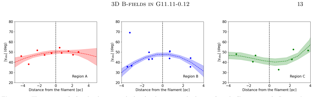
The inferred inclinations rise toward the filament spine in Regions A and B, which the authors interpret as an arc-shaped 3D field wrapping the filament, and drop in Region C, interpreted as gravitational back-and-forth bending.
The same modeling chain constrains dust properties in the outer regions: maximum grain size ~0.25 μm and elongation s ≳ 1.4 — diffuse-ISM-like values implying little grain growth so far in G11.
The method is portable: the authors identify other filamentary clouds (nearby and distant) as next targets, making archival polarimetry a resource for multi-scale 3D field maps.

Reading between the lines

Editorial extensions of the paper, not claims the author makes directly.

My extension: the real payoff is archival. Any cloud that already has starlight polarimetry, a column-density map, and an angle-dispersion map is, in principle, ready for a 3D field map; the bottleneck shifts from observing time to the reliability of the alignment model.
My extension: the degeneracy reported in Sec. 7.4 makes a sharp prediction — if grains are more elongated (s ≈ 2) and less efficiently aligned (weak iron inclusions) than assumed, the inferred rise of |γ| toward the spine would shrink or invert; comparing inferred angles against an independent probe would settle which model is right.
My extension: only |γ| is recovered, so the same arc could be curved toward or away from the observer; combining the inclination maps with sign-sensitive measurements (Zeeman or Faraday rotation) and gas radial-velocity gradients could fix the orientation and distinguish shock-wrapped fields from gravity-dragged accretion flow.

Share X Bluesky LinkedIn Reddit HN

Signed reviews

No signed human review yet.

Editorial analysis

A structured set of objections, weighed in public.

Desk editor's note, referee report, and a circularity audit.

Desk Editor's Note

read the letter

First, what you should know: this is the first real-data application of Hoang and Truong's starlight-polarization technique for 3D magnetic field inclination estimates, applied to the G11 filament. It is transparent about its inputs and limitations, and the derived dust properties (amax ~0.25 micron, s >=1.4) are consistent with independent benchmarks. But the headline claim of a local 3D arc-shaped field is softer than the abstract implies. The paper's own Section 7.4 demonstrates a degeneracy between geometry and grain-alignment efficiency: the same observed maximum polarization efficiency can be reproduced with (s=1.4, N_cl > 5000), (s=1.6, N_cl = 1200), or (s=2.0, N_cl = 130), and the authors state the inferred dense-region angles would increase accordingly. Since the arc-shaped morphology is exactly an increase of |gamma| toward the spine, the current analysis does not uniquely separate geometry from alignment systematics. That is not an external criticism; it is written in the paper.

Equally important, there are numeric inconsistencies: Section 7.2 quotes Region D at ~64 degrees while Table 2 says 48.6 and Fig. 10's color scale stops at 55; the mean inclination flips between 48 and 50 across abstract and body. These need to be corrected. The calibration anchor at the 99th percentile of polarization efficiency assumes ideal geometry and zero turbulence there, and no systematic error budget is propagated.

What it does well: the formalism is clean (Eq. 6 follows from Eq. 3), the observational data sets are public and used carefully, and the MRAT modeling is done with an open-source code. The paper is honest about its assumptions, which is more than many first-application papers do.

Bottom line: this is a conditional result. The 3D field strength estimate (B3D ~ 80-150 microgauss; factor 1.3-1.35 over POS) is more robust because it only depends on sin gamma, but the arc-shaped morphology claim is not. I would send it to peer review, but the authors need to present angle maps under the MRAT scenarios of Table 3, quantify the anchor's effect, and fix the inconsistent numbers. If they do that, this becomes a useful demonstration of the technique's potential and its limits. Target audience: observers and theorists working on magnetic field probing; good for a reading group discussion on degeneracies.

Referee Report

2 major / 5 minor

Summary. This paper presents the first application of the Truong & Hoang (2025) technique to infer 3D magnetic-field inclination angles from starlight polarization efficiency, applied to the massive IRDC filament G11.11-0.12. Using archival Ks-band SIRPOL polarimetry (Chen et al. 2023), Gaia-derived R_V extinction data (Zhang & Green 2025), and Herschel-derived column density/temperature maps (Zucker et al. 2018), the authors constrain the maximum grain size (~0.25 micron) and grain axial ratio (s ≳ 1.4), compute radiative-torque alignment maps (a_align, f_pol), and derive |γ| via Eq. (6) after correcting for magnetic turbulence. They report a mean inclination angle of ~48–50°, infer an arc-shaped 3D B-field morphology in Regions A and B, and derive B_3D = 80–150 µG, implying sub-Alfvénic and mostly sub-critical conditions. The paper is transparent about its inputs and includes an MRAT/iron-inclusion sensitivity analysis in Sec. 7.4.

Significance. The method is potentially significant: if validated, it would show that archival starlight polarimetry plus modern RAT/MRAT alignment theory can recover LOS magnetic-field inclination angles and 3D morphology in a massive filament, complementing Faraday-rotation/Zeeman methods. The paper's strengths include a clear algebraic framework (Eq. 6), use of external publicly available data, a public modeling code (DustPOL_py), and an explicit discussion of MRAT degeneracies. The derived dust properties are consistent with independent diffuse-ISM benchmarks. However, the central morphological claim (arc-shaped fields) is currently entangled with a recognized geometry-versus-alignment degeneracy, and the quantitative outputs lack propagated systematics. The significance is therefore real but conditional on resolving that degeneracy.

major comments (2)

[Sec. 6.2, Fig. 11, and Eq. (6)] The central claim of local arc-shaped B-fields in Regions A and B rests on the rise of |γ| toward the spine. This is not uniquely decoupled from the grain-alignment model. Eq. (6) computes sin^2γ by dividing the observed P_K/N_H by the ideal-RAT products P_i/N_H and f_pol, with R=1 and uniform (a_max=0.25 μm, s=1.4) fixed in Secs. 4–5. If MRAT alignment is less efficient in the denser spine, f_pol is overestimated there, inflating the inferred |γ| exactly where the arc signal appears. Sec. 7.4 and Table 3/Fig. 15 show the same observed maximum is reproduced by (s=1.4, N_cl>5000), (s=1.6, N_cl=1200), and (s=2.0, N_cl=130), and the authors state that dense-region angles are expected to increase due to degeneracy with reduced MRAT alignment efficiency. The arc-shaped signal in Fig. 11 has the same sign as this degeneracy. To support the abstract/Sec. 6.2 claim, the authors should either joi
[Secs. 4.1.2–5 and Tables 1–2] The quantitative outputs (mean |γ| ~50°, B_3D = 80–150 μG, M_A, μ_φ) are point estimates with no propagation of input systematics. a_max is inferred from the observed R_V range (2.65–2.95) in Fig. 5; s is anchored to the 99th-percentile maximum under the ideal-geometry assumption in Sec. 4.3; W=5 pc is assumed in Eq. (10); and γ_rad, λ̄, and R are adopted without uncertainties in Sec. 4.2.3. These quantities enter multiplicatively in Eq. (6) through P_i/N_H and f_pol, so a 10–20% systematic in these inputs shifts |γ| by several degrees and B_3D by tens of μG. Please provide a systematic-error budget or bracketing calculations; otherwise the reported means in Table 2 cannot be quantitatively compared with theory or other observations.

minor comments (5)

[Sec. 7.2 / Table 2] The text states that Region D has a mean inclination angle of ~64°, but Table 2 reports 48.6°. These values should be reconciled.
[Abstract / Sec. 6.1] The abstract gives a mean angle of ~48°, while Sec. 6.1 quotes ~50° and Table 2 gives region means of 43.9–49.2°. State the aggregation method and use one consistent value.
[Sec. 3.2] A resolution of 43″ at 3.6 kpc corresponds to roughly 0.75 pc, not 1.4 pc as written. Please check the conversion.
[Fig. 15 caption] The third panel's caption contains 'SPM, N_cl = 30, α=0.93', while the text and panel title use N_cl=130, s=2.0. This appears to be a typo.
[Sec. 4.3 and Fig. 8] Please state the number of stars used to define the 99th-percentile maximum and clarify whether the anchor is the 99th percentile of the binned running mean or of the unbinned sample.

Circularity Check

0 steps flagged · score 1.0 of 10

No significant circularity; the 3D inclination inference is a model-calibrated inversion of external polarization data, not a renaming of fitted parameters.

full rationale

The derivation chain is not circular. The dust extinction constraint amax=0.25 micron comes from the independent Gaia-based RV map (Zhang & Green 2025), and the elongation s~1.4 is calibrated by matching the modeled maximum polarization efficiency to the observed 99th-percentile value under an explicitly stated geometric assumption (gamma=90, Fturb=1) at a single anchor point. This is a normalization/calibration, not a fit of the inclination-angle map that is later claimed as a prediction. The inferred inclination map then follows from Eq. (6), with f_pol computed from the RAT/MRAT alignment model using Herschel-derived n(H2) and Td maps and Fturb computed from the observed position-angle dispersion; these inputs are independent of the inclination values. The arc-shaped morphology in Regions A and B is a spatial trend of gamma relative to the filament spine, i.e., a residual after applying the alignment and turbulence corrections, not the calibration parameter itself. Section 7.4 does expose a degeneracy between the number of iron inclusions, grain elongation, and the inferred dense-region angles, but this is model uncertainty/limitation, not circularity: multiple (s, Ncl) models reproduce the same maximum efficiency and would change the magnitudes of the inferred angles, but the paper does not claim uniqueness. The self-citations to Truong & Hoang (2025) and Hoang & Truong (2024) supply the inversion method and synthetic validation from the same group, but the equations are physically derived and the target data are external archival observations (Chen et al. 2023, Gaia/Herschel products), so this is normal series practice rather than load-bearing circularity. No step equates a fitted parameter with the claimed prediction by construction.

Assumptions & free parameters 8 free parameters · 6 assumptions · 1 invented entities

The inversion rests on roughly eight numbers chosen or fitted by the authors. amax and s are fit to observations (Gaia RV; the 99th-percentile maximum polarization efficiency under an assumed ideal geometry), W, gamma_rad, lambda_bar, and R/Ncl are adopted values from the authors' own alignment framework, and beta and Md/g are standard ISM inputs. The algebra of Eqs. 1-6 is clean; the fragile part is the chain of assumptions converting a polarization-efficiency map into an angle map. No new particles or forces are introduced.

free parameters (8)

amax (maximum grain size) = 0.25 micron (mean)
Fit to the Gaia-based RV ~ 2.65-2.95 (Sec. 4.1.2, Fig. 5). Sets the upper cutoff of the MRN size distribution and thereby Pi/NH and the extinction curve shape used in the inversion.
s (grain axial ratio) = 1.4 (quoted as lower limit s >= 1.4, then used as fixed value)
Calibrated in Sec. 4.3 / Fig. 8 by matching modeled (PK/NH)mod to the observed 99th-percentile maximum under assumed ideal geometry (sin^2 gamma = 1, Fturb = 1); directly sets Pi/NH = 3.02e-22 % cm^2 in Sec. 5.
99th-percentile anchor = (PK/NH)max ~ 2.3e-22 % cm^2
Hand-chosen data cut defining the 'maximum polarization efficiency' used both for the s-calibration and as the reference point of the gamma inversion (Sec. 4.3, Fig. 8 left).
filament width W = 5 pc
Assumed cylindrical depth for converting NH2 to nH2 via nH2 = NH2/W (Eq. 10, Sec. 4.2.2), taken from Kainulainen et al. 2013; enters aalign (Eq. B6) and hence fpol.
ISRF anisotropy and mean wavelength (gamma_rad, lambda_bar) = 0.1 and 1.2 micron
Assumed typical interstellar radiation-field parameters (Sec. 4.2.3) entering the aalign formula (Eq. B6); no local radiation-field modeling is performed for G11.
Rayleigh reduction factor R / iron-cluster parameters = R = 1 baseline; Ncl in {>5000, 1200, 130}, phi_sp = 0.01 in MRAT scenarios
Headline angles assume perfect alignment of large grains (R = 1). Sec. 7.4 explores SPM grains with iron inclusions; the same observed maximum is matched by (s = 1.4, Ncl > 5000), (s = 1.6, Ncl = 1200), or (s = 2.0, Ncl = 130), making the alignment efficiency degenerate with grain shape.
turbulence factor model = Fturb ~ 1 - 1.5 sin^2(sigma_theta), isotropy assumed
The POS polarization-angle dispersion sigma_theta from 2'x2' cells is assumed to fully describe 3D field tangling for depolarization (Eq. 7, Eq. C10, Sec. 3.3); anisotropic turbulence would bias Fturb and hence all inferred angles.
MRN power-law index and dust-to-gas ratio (beta, Md/g) = beta = 3.5, Md/g = 0.01
Adopted standard diffuse-ISM values (Mathis et al. 1977; Table 4) that set the Astrodust size-distribution normalization and therefore the absolute scale of Pi/NH.

assumptions (6)

domain assumption RAT/MRAT alignment theory quantitatively predicts falign(a) from local environmental parameters (Eqs. 9, B6-B9).
The physics backbone of the inversion: aalign, fhigh-J, and R are taken from Lazarian & Hoang 2007; Hoang & Lazarian 2008, 2016. The theory is community-accepted, but the specific parameterization used here (SPM iron inclusions, delta_mag) comes from the authors' own works.
domain assumption Optically thin polarization-efficiency decomposition with a single mean field direction: PK/NH = (Pi/NH) fpol Fturb sin^2 gamma (Eqs. 1-3).
Assumes one dominant field component per sightline and that all small-scale tangling is absorbed by Fturb; multi-component or strongly curved fields along the LOS would break the sin^2 gamma scaling. This is the foundational equation from Truong & Hoang 2025.
domain assumption Isotropic magnetic turbulence: POS polarization-angle dispersion sigma_theta fully determines the 3D depolarization factor Fturb (Eq. 7 to Eq. C10).
If the turbulence is anisotropic, Fturb computed from POS angles is biased, which shifts the inferred gamma everywhere (Sec. 3.3).
ad hoc to paper Dust properties are uniform across the outer regions: amax = 0.25 micron, s = 1.4, and Pi/NH is constant (Sec. 5).
Stated in Sec. 5 and discussed in Sec. 7.3, where the authors themselves acknowledge that anisotropic grain growth (increasing amax and s with density) would modify the inferred angles. The arc-shaped trend toward the spine is not robust to this premise.
ad hoc to paper The maximum observed polarization efficiency occurs at ideal geometry: sin^2 gamma = 1 and Fturb = 1 (Sec. 4.3).
Calibration anchor for the grain-elongation fit. Unfalsifiable within the paper and systematically shifts every inferred |gamma_obs| if the true field at the 99th-percentile pixel is inclined or tangled; its error budget is never quantified.
domain assumption Astrodust + PAH composition with MRN power law and two log-normal PAH modes (Appendix A, Table 4), with cross-sections from Draine & Hensley 2021b and Hensley & Draine 2023.
Adopted dust model; grain composition, porosity, and optical constants are inputs from prior literature, not tested against G11-specific emission or scattering data.

invented entities (1)

Arc-shaped 3D B-field morphology (illustrated in Fig. 12)
purpose: Interpretive geometric model organizing the inferred |gamma_obs| profiles in Regions A, B, and C of G11.
This is not a new physical entity but a sketch of the inferred field geometry; it has two equally allowed signs (folded toward or away from the observer) and no independent observational handle in this paper (the authors suggest Zeeman or Faraday measurements for future confirmation).

how reviews work

0 comments

Cite this review

Pith. "Pith review of 3D B-fieLds in the InterStellar medium and Star-forming regions (3D-BLISS): I. Using Starlight Polarization in the Massive IRDC Filament G11.11-0.12." pith.science (2026). https://pith.science/paper/7QIQ4UXO

@misc{pith2026251006726,
  author       = {Pith},
  title        = {Pith review of: 3D B-fieLds in the InterStellar medium and Star-forming regions (3D-BLISS): I. Using Starlight Polarization in the Massive IRDC Filament G11.11-0.12},
  year         = {2026},
  howpublished = {\url{https://pith.science/paper/7QIQ4UXO}},
  note         = {Machine review of arXiv:2510.06726}
}

abstract

Measuring three-dimensional magnetic fields (3D B-fields) is essential to understand the formation and evolution of the interstellar medium and multi-scale star formation; however, the accurate measurement of 3D B-fields is still challenging. The dust polarization angles by magnetically aligned grains provide the projected B-fields onto the plane-of-sky, while the dust polarization degree provides the B-field's inclination angle with respect to the line-of-sight. Our previous theoretical studies proposed a new method of probing 3D B-fields using dust polarization combined with the Radiative Torque (RAT) alignment theory and demonstrated the accurate inference of B-field inclination angles using synthetic polarization data. In this paper, we report the first application of the new technique to study 3D B-fields and dust properties in the G11.11-0.12 filament (hereafter G11) from starlight polarization observations taken by ISRF/SIRPOL at $2.19\,\rm\mu m$. Using both observed starlight polarization and optical dust extinction curves from the Gaia mission, we constrained the maximum grain size of $0.25\,\rm\mu m$ and the grain elongation with an axial ratio of $s\gtrsim 1.4$ in the outer regions of G11. We calculated the alignment properties in G11 by using the \textsc{DustPOL\_py} code. The B-field's inclination angles in G11 are then inferred from the observed starlight polarization efficiency when the grain alignment is included, with a mean angle of $\sim 48$ degrees. From these inferred inclination angles, we found evidence of the local 3D arc-shaped B-field structure toward the sightline. These findings are important for understanding 3D B-field's roles in the formation and evolution of massive filamentary clouds.

Figures

Figures reproduced from arXiv: 2510.06726 by the authors.

**Figure 1.** The foreground-corrected Ks-band polarization measured by SIRPOL at 2.19 µm (blue segments, see Chen et al. 2023), also indicating the orientation of POS B-fields in the outer regions of G11. The length of the blue segments is in an arbitrary scale. The polarization vectors are overplotted onto a gray map of molecular hydrogen column density NH2 derived from Herschel observations (Zucker et al. 2018). The massive c… view at source ↗

**Figure 2.** The starlight polarization efficiency PK/NH vs. the molecular hydrogen column density NH2 in four subregions along the spine of the G11 filament. A power-law fit is applied to the running mean of the observed data [PITH_FULL_IMAGE:figures/full_fig_p006_2.png] view at source ↗

**Figure 3.** The spatial distribution of the magnetic turbulence factor Fturb calculated from the polarization angle dispersion in each grid cell spacing of 2′ × 2 ′ (see also Chen et al. 2023) by using the unsharp-masking method (Pattle et al. 2017). PAHs model was applied to explain the extinction, emission, and polarization observations in the diffuse ISM by Hensley & Draine (2023). We consider the grains to have an oblate … view at source ↗

Figures from the paper (12 more)

**Figure 5.** Figure 5: The variation of the modeled RV generated by DustPOL py for Astrodust+PAHs grains, considering varying maximum grain size amax and grain axial ratio of oblate spheroids s > 1. The RV increases with increasing amax. The modeled RV is best-fitted to the observed one when…

**Figure 4.** Figure 4: The spatial distribution of the total-to-selective extinction ratio RV in the outer regions of G11 derived from interstellar dust extinction data from background stars provided by the Gaia mission (Zhang & Green 2025). The observed RV is around 2.65 - 2.95 RV charact…

**Figure 6.** Figure 6: Maps of the volume density nH2 (left panel) and the dust temperature Td (right panel) derived from multi-wavelength Herschel observations at 160, 250, 350, and 500 µm (see Zucker et al. 2018). the G11 and the modeled profile numerically calculated by the DustPOL py cod…

**Figure 7.** Figure 7: Map of the minimum aligned size aalign induced by RATs from interstellar radiation fields in the outer regions of G11. alignment by RATs (Pi,K/NH and fpol,K, see Section 5) and magnetic turbulence (Fturb, see Section 3.3) within the G11 filament, we derive the local 3D…

**Figure 8.** Figure 8: Left panel: Histogram of the observed starlight polarization efficiency PK/NH in the G11 filament by Chen et al. (2023). The 99th percentile of the data (∼ 2.3 × 10−22 % cm2 ) is marked by a dashed black vertical line. Right panel: The comparison between the observed a…

**Figure 9.** Figure 9: Map of the polarization coefficient fraction fpol,K at Ks band derived from the local RAT alignment properties and the constrained intrinsic dust properties in the G11. The fpol,K decreases toward the denser filament due to the grain alignment loss by increasing gas ra…

**Figure 11.** Figure 11: The variation of inferred inclination angles |γobs| with respect to the distance from the filament spine for Regions A (left panel), B (middle panel), and C (right panel). A polynomial fit is applied to fit the data with 1σ uncertainty (color shade regions). 𝑥ො yො zො …

**Figure 12.** Figure 12: Illustration of the morphology of 3D B-fields in Regions A, B and C of the G11 filament derived from the inferred inclination angles in two scenarios: (a) 3D B-fields are curved toward the observer with the positive γobs and (b) 3D B-fields are curved away from the ob…

**Figure 13.** Figure 13: The spatial distribution of the local 3D B-field strength B3D in each 2′ × 2 ′ grid cell in the G11 filament. Galactic plane CO survey using the 13.7 m telescope of the Purple Mountain Observatory (see Su et al. 2019). The mean velocity dispersion σv in each cell of 2…

**Figure 14.** Figure 14: The maps of the Alfv´enic Mach MA,3D (left panel) and the critical mass-to-flux ratio µϕ,3D (right panel) derived from the local 3D B-field strength B3D. 7.2. Implications of 3D B-fields Morphology for Understanding Filament Evolution From the local 3D inclination ang…

**Figure 15.** Figure 15: Observed polarization efficiency vs. the modeled one (PK/NH)mod generated by the DustPOL py code, but considering MRAT alignment for SPM grains with varying number of iron inclusions Ncl and grain elongations s. The ideal conditions of B-fields are considered at the m…

**Figure 16.** Figure 16: The normalized dust extinction curve Aλ/NH at optical-NIR wavelengths (λ = 0.1 − 20 µm) modeled by DustPOL py code for Astrodust+PAHs grains. Varying amax (left panel) and axial ratios of oblate grains (right panel) are assumed. C. EFFECT OF MAGNETIC TURBULENCE ON TH…

Discussion (0). Continue with ORCID to comment.

Reference graph

Works this paper leans on

122 extracted references · 1 linked inside Pith

[1]

- [1] #1 = = ^ ^ ^ .\!\!^ d .\!\!^ h .\!\!^ m .\!\!^ s .\!\!^ @mss

thebibliography [1] 20pt to REFERENCES 6pt =0pt 10pt plus 3pt =0pt =0pt =1pt plus 1pt =0pt =0pt -12pt =13pt plus 1pt =20pt =13pt plus 1pt \@M =10000 =-1.0em =0pt =0pt 0pt =0pt =1.0em @enumiv\@empty 10000 10000 `\.\@m \@noitemerr \@latex@warning Empty `thebibliography' environment \@ifnextchar \@reference \@latexerr Missing key on reference command Each re...

2019
[2]

, " * write output.state after.block = add.period write newline

ENTRY address author booktitle chapter edition editor howpublished institution journal key month note number organization pages publisher school series title type volume year label extra.label sort.label short.list INTEGERS output.state before.all mid.sentence after.sentence after.block FUNCTION init.state.consts #0 'before.all := #1 'mid.sentence := #2 '...
[3]

write newline

" write newline "" before.all 'output.state := FUNCTION n.dashify 't := "" t empty not t #1 #1 substring "-" = t #1 #2 substring "--" = not "--" * t #2 global.max substring 't := t #1 #1 substring "-" = "-" * t #2 global.max substring 't := while if t #1 #1 substring * t #2 global.max substring 't := if while FUNCTION word.in bbl.in " " * FUNCTION format....
[4]

J., Tielens , A

Allamandola , L. J., Tielens , A. G. G. M., & Barker , J. R. 1985, , 290, L25

1985
[5]

G., Lazarian , A., & Vaillancourt , J

Andersson , B. G., Lazarian , A., & Vaillancourt , J. E. 2015, , 53, 501

2015
[6]

Angarita , Y., Versteeg , M. J. F., Haverkorn , M., et al. 2023, , 166, 34

2023
[7]

M., Sip o cz , B

Astropy Collaboration , Price-Whelan , A. M., Sip o cz , B. M., et al. 2018, , 156, 123

2018
[8]

2024, Universe, 10, 218

Basu , S., Li , X., & Bino , G. 2024, Universe, 10, 218

2024

Show all 122 references

[9]

Bate , M. R. 2022, , 514, 2145

2022
[10]

2015, , 24, 4

Beck , R. 2015, , 24, 4

2015
[11]

A., Clayton , G

Cardelli , J. A., Clayton , G. C., & Mathis , J. S. 1989, , 345, 245

1989
[12]

1953, , 118, 113

Chandrasekhar , S., & Fermi , E. 1953, , 118, 113

1953
[13]

K., Li , Z.-Y., Fissel , L

Chen , C.-Y., King , P. K., Li , Z.-Y., Fissel , L. M., & Mazzei , R. R. 2019, , 485, 3499

2019
[14]

2023, The Role of Magnetic Fields in the Formation of the Filamentary Infrared Dark Cloud G11.11-0.12

Chen, Z., Sefako, R., Yang, Y., et al. 2023, The Role of Magnetic Fields in the Formation of the Filamentary Infrared Dark Cloud G11.11-0.12

2023
[15]

2023, , 525, 107

Chen , Z., Sefako , R., Yang , Y., et al. 2023, , 525, 107

2023
[16]

2022, Research in Astronomy and Astrophysics, 22, 075017

Chen , Z., Sefako , R., Yang , Y., et al. 2022, Research in Astronomy and Astrophysics, 22, 075017

2022
[17]

2022, , 941, 122

Ching , T.-C., Qiu , K., Li , D., et al. 2022, , 941, 122

2022
[18]

P., Tassis , K., & Goldsmith , P

Clemens , D. P., Tassis , K., & Goldsmith , P. F. 2016, , 833, 176

2016
[19]

Crutcher , R. M. 1999, , 520, 706

1999
[20]

Crutcher , R. M. 2012, , 50, 29

2012
[21]

M., Nutter , D

Crutcher , R. M., Nutter , D. J., Ward-Thompson , D., & Kirk , J. M. 2004, , 600, 279

2004
[22]

1951, Physical Review, 81, 890

Davis , L. 1951, Physical Review, 81, 890

1951
[23]

K., Bhadari , N

Dewangan , L. K., Bhadari , N. K., Maity , A. K., et al. 2024, , 527, 5895

2024
[24]

S., et al

Doi , Y., Nakamura , K., Kawabata , K. S., et al. 2024, , 961, 13

2024
[25]

Draine , B. T. 2006, , 636, 1114

2006
[26]

Draine , B. T. 2011, Physics of the Interstellar and Intergalactic Medium

2011
[27]

Draine , B. T. 2024 a , , 961, 103

2024
[28]

Draine , B. T. 2024 b , , 969, 92

2024
[29]

T., & Fraisse , A

Draine , B. T., & Fraisse , A. A. 2009, , 696, 1

2009
[30]

T., & Hensley , B

Draine , B. T., & Hensley , B. S. 2021 a , , 909, 94

2021
[31]

T., & Hensley , B

Draine , B. T., & Hensley , B. S. 2021 b , , 919, 65

2021
[32]

T., & Li , A

Draine , B. T., & Li , A. 2007, , 657, 810

2007
[33]

T., Li , A., Hensley , B

Draine , B. T., Li , A., Hensley , B. S., et al. 2021, , 917, 3

2021
[34]

T., & Salpeter , E

Draine , B. T., & Salpeter , E. E. 1979, , 231, 77

1979
[35]

H., Crutcher , R

Falgarone , E., Troland , T. H., Crutcher , R. M., & Paubert , G. 2008, , 487, 247

2008
[36]

Gaia Collaboration , Vallenari , A., Brown , A. G. A., et al. 2023, , 674, A1

2023
[37]

C., & Hoang , T

Giang , N. C., & Hoang , T. 2024, , 530, 984

2024
[38]

C., Hoang , T., Kim , J.-G., & Tram , L

Giang , N. C., Hoang , T., Kim , J.-G., & Tram , L. N. 2023, , 520, 3788

2023
[39]

C., V \'a zquez-Semadeni , E., & Zamora-Avil \'e s , M

G \'o mez , G. C., V \'a zquez-Semadeni , E., & Zamora-Avil \'e s , M. 2018, , 480, 2939

2018
[40]

F., & Lazarian , A

Gonz \'a lez-Casanova , D. F., & Lazarian , A. 2017, , 835, 41

2017
[41]

2018, , 610, A16

Guillet , V., Fanciullo , L., Verstraete , L., et al. 2018, , 610, A16

2018
[42]

Hall , J. S. 1949, Science, 109, 166

1949
[43]

R., Millman , K

Harris , C. R., Millman , K. J., van der Walt , S. J., et al. 2020, , 585, 357

2020
[44]

2010, , 518, L95

Henning , T., Linz , H., Krause , O., et al. 2010, , 518, L95

2010
[45]

S., & Draine , B

Hensley , B. S., & Draine , B. T. 2023, , 948, 55

2023
[46]

Hildebrand, R. H. 1988, Royal Astronomical Society, Quarterly Journal (ISSN 0035-8738), vol. 29, Sept. 1988, p. 327-351., 29, 327

1988
[47]

Hiltner , W. A. 1949, Science, 109, 165

1949
[48]

2012, , 422, 1263

Hirashita , H. 2012, , 422, 1263

2012
[49]

2022, , 928, 102

Hoang , T. 2022, , 928, 102

2022
[50]

2008, , 388, 117

Hoang , T., & Lazarian , A. 2008, , 388, 117

2008
[51]

2014, , 438, 680

Hoang , T., & Lazarian , A. 2014, , 438, 680

2014
[52]

2016, , 831, 159

Hoang , T., & Lazarian , A. 2016, , 831, 159

2016
[53]

N., Lee , H., Diep , P

Hoang , T., Tram , L. N., Lee , H., Diep , P. N., & Ngoc , N. B. 2021, , 908, 218

2021
[54]

N., Minh Phan , V

Hoang , T., Tram , L. N., Minh Phan , V. H., et al. 2022, , 164, 248

2022
[55]

2024, , 965, 183

Hoang , T., & Truong , B. 2024, , 965, 183

2024
[56]

2025, arXiv e-prints, arXiv:2505.07422

Hu , Y. 2025, arXiv e-prints, arXiv:2505.07422

2025 arXiv
[57]

2023 a , , 524, 4431

Hu , Y., & Lazarian , A. 2023 a , , 524, 4431

2023
[58]

2023 b , , 524, 4431

Hu , Y., & Lazarian , A. 2023 b , , 524, 4431

2023
[59]

2023 c , , 524, 2379

Hu , Y., & Lazarian , A. 2023 c , , 524, 2379

2023
[60]

2024, , 527, 11240

Hu , Y., Lazarian , A., Wu , Y., & Fu , C. 2024, , 527, 11240

2024
[61]

Hunter , J. D. 2007, Computing in Science and Engineering, 9, 90

2007
[62]

W., Kim , J., Chung , E

Hwang , J., Lee , C. W., Kim , J., Chung , E. J., & Kim , K.-T. 2024, , 974, 231

2024
[63]

2018, , 70, S53

Inoue , T., Hennebelle , P., Fukui , Y., et al. 2018, , 70, S53

2018
[64]

2015, , 580, A49

Inutsuka , S.-i., Inoue , T., Iwasaki , K., & Hosokawa , T. 2015, , 580, A49

2015
[65]

2015, , 584, A94

Juvela , M., Demyk , K., Doi , Y., et al. 2015, , 584, A94

2015
[66]

E., Henning , T., & Stutz , A

Kainulainen , J., Ragan , S. E., Henning , T., & Stutz , A. 2013, , 557, A120

2013
[67]

2006, in Society of Photo-Optical Instrumentation Engineers (SPIE) Conference Series, Vol

Kandori , R., Kusakabe , N., Tamura , M., et al. 2006, in Society of Photo-Optical Instrumentation Engineers (SPIE) Conference Series, Vol. 6269, Ground-based and Airborne Instrumentation for Astronomy, ed. I. S. McLean & M. Iye , 626951

2006
[68]

2017, , 848, 110

Kandori , R., Tamura , M., Tomisaka , K., et al. 2017, , 848, 110

2017
[69]

2018, , 865, 121

Kandori , R., Tomisaka , K., Tamura , M., et al. 2018, , 865, 121

2018
[70]

L., Evans , II, N

Kauffmann , J., Bertoldi , F., Bourke , T. L., Evans , II, N. J., & Lee , C. W. 2008, , 487, 993

2008
[71]

2007, , 378, 910

Lazarian , A., & Hoang , T. 2007, , 378, 910

2007
[72]

2008, , 676, L25

Lazarian , A., & Hoang , T. 2008, , 676, L25

2008
[73]

2020, , 896, 44

Lee , H., Hoang , T., Le , N., & Cho , J. 2020, , 896, 44

2020
[74]

M., & Draine , B

Lee , H. M., & Draine , B. T. 1985, , 290, 211

1985
[75]

Leger , A., & Puget , J. L. 1984, , 137, L5

1984
[76]

K., Inoue , T., Fukui , Y., et al

Maity , A. K., Inoue , T., Fukui , Y., et al. 2024, , 974, 229

2024
[77]

S., Mezger , P

Mathis , J. S., Mezger , P. G., & Panagia , N. 1983, , 128, 212

1983
[78]

S., Rumpl , W., & Nordsieck , K

Mathis , J. S., Rumpl , W., & Nordsieck , K. H. 1977, , 217, 425

1977
[79]

2023, , 674, A3

Montegriffo , P., De Angeli , F., Andrae , R., et al. 2023, , 674, A3

2023
[80]

2018, , 56, 41

Motte , F., Bontemps , S., & Louvet , F. 2018, , 56, 41

2018
[81]

2003, in Society of Photo-Optical Instrumentation Engineers (SPIE) Conference Series, Vol

Nagayama , T., Nagashima , C., Nakajima , Y., et al. 2003, in Society of Photo-Optical Instrumentation Engineers (SPIE) Conference Series, Vol. 4841, Instrument Design and Performance for Optical/Infrared Ground-based Telescopes, ed. M. Iye & A. F. M. Moorwood , 459--464

2003
[82]

1978, , 30, 671

Nakano , T., & Nakamura , T. 1978, , 30, 671

1978
[83]

B., Diep , P

Ngoc , N. B., Diep , P. N., Hoang , T., et al. 2023, , 953, 66

2023
[84]

C., Stone , J

Ostriker , E. C., Stone , J. M., & Gammie , C. F. 2001, , 546, 980

2001
[85]

2021 a , , 651, A116

Padovani , M., Bracco , A., Jeli \'c , V., Galli , D., & Bellomi , E. 2021 a , , 651, A116

2021
[86]

2018, , 620, L4

Padovani , M., & Galli , D. 2018, , 620, L4

2018
[87]

K., & Fontani , F

Padovani , M., Marcowith , A., Galli , D., Hunt , L. K., & Fontani , F. 2021 b , , 649, A149

2021
[88]

2015, , 452, 715

Panopoulou , G., Tassis , K., Blinov , D., et al. 2015, , 452, 715

2015
[89]

V., Psaradaki , I., & Tassis , K

Panopoulou , G. V., Psaradaki , I., & Tassis , K. 2016, , 462, 1517

2016
[90]

2019, Frontiers in Astronomy and Space Sciences, 6, 15

Pattle , K., & Fissel , L. 2019, Frontiers in Astronomy and Space Sciences, 6, 15

2019
[91]

2017, , 846, 122

Pattle , K., Ward-Thompson , D., Berry , D., et al. 2017, , 846, 122

2017
[92]

Pillai , T., Kauffmann , J., Wiesemeyer , H., & Menten , K. M. 2016, , 591, A19

2016
[93]

Pillai , T. G. S., Clemens , D. P., Reissl , S., et al. 2020, Nature Astronomy, 4, 1195

2020
[94]

Planck Collaboration , Ade , P. A. R., Aghanim , N., et al. 2015, , 576, A104

2015
[95]

2020, , 641, A12

Planck Collaboration , Aghanim , N., Akrami , Y., et al. 2020, , 641, A12

2020
[96]

M., Brauer , R., et al

Reissl , S., Stutz , A. M., Brauer , R., et al. 2018, , 481, 2507

2018
[97]

G., et al

Soam , A., Liu , T., Andersson , B. G., et al. 2019, , 883, 95

2019
[98]

2019, , 240, 9

Su , Y., Yang , J., Zhang , S., et al. 2019, , 240, 9

2019
[99]

2019, , 71, S7

Sugitani , K., Nakamura , F., Shimoikura , T., et al. 2019, , 71, S7

2019
[100]

2022, Frontiers in Astronomy and Space Sciences, 9, 940027

Tahani , M. 2022, Frontiers in Astronomy and Space Sciences, 9, 940027

2022
[101]

C., & Kainulainen , J

Tahani , M., Plume , R., Brown , J. C., & Kainulainen , J. 2018, , 614, A100

2018
[102]

C., Soler , J

Tahani , M., Plume , R., Brown , J. C., Soler , J. D., & Kainulainen , J. 2019, , 632, A68

2019
[103]

2022, , 660, L7

Tahani , M., Glover , J., Lupypciw , W., et al. 2022, , 660, L7

2022
[104]

2024, , 687, A18

Tapinassi , D., Galli , D., Padovani , M., & Beuther , H. 2024, , 687, A18

2024
[105]

N., & Hoang , T

Tram , L. N., & Hoang , T. 2022, Frontiers in Astronomy and Space Sciences, 9, 923927

2022
[106]

N., Hoang , T., Lee , H., et al

Tram , L. N., Hoang , T., Lee , H., et al. 2021, , 906, 115

2021
[107]

N., Hoang , T., Soam , A., Lesaffre , P., & Reach , W

Tram , L. N., Hoang , T., Soam , A., Lesaffre , P., & Reach , W. T. 2020, , 893, 138

2020
[108]

N., Hoang , T., Wiesemeyer , H., et al

Tram , L. N., Hoang , T., Wiesemeyer , H., et al. 2024, , 689, A290

2024
[109]

N., Hoang , T., Lazarian , A., et al

Tram , L. N., Hoang , T., Lazarian , A., et al. 2025, arXiv e-prints, arXiv:2501.16079

2025
[110]

2025, , 981, 83

Truong , B., & Hoang , T. 2025, , 981, 83

2025
[111]

E., Andersson , B

Vaillancourt , J. E., Andersson , B. G., Clemens , D. P., et al. 2020, , 905, 157

2020
[112]

E., et al

Virtanen , P., Gommers , R., Oliphant , T. E., et al. 2020, Nature Methods, 17, 261

2020
[113]

P., et al

Wang , J.-W., Lai , S.-P., Clemens , D. P., et al. 2020, , 888, 13

2020
[114]

2017, , 849, 157

Wang , J.-W., Lai , S.-P., Eswaraiah , C., et al. 2017, , 849, 157

2017
[115]

2014, , 439, 3275

Wang , K., Zhang , Q., Testi , L., et al. 2014, , 439, 3275

2014
[116]

Wang , S., Li , A., & Jiang , B. W. 2015, , 811, 38

2015
[117]

C., & Draine , B

Weingartner , J. C., & Draine , B. T. 2001, , 553, 581

2001
[118]

Whittet , D. C. B., Hough , J. H., Lazarian , A., & Hoang , T. 2008, , 674, 304

2008
[119]

Zhang , X., & Green , G. M. 2025, Science, 387, 1209

2025
[120]

M., & Rix , H.-W

Zhang , X., Green , G. M., & Rix , H.-W. 2023, , 524, 1855

2023
[121]

2018, , 864, 153

Zucker , C., Battersby , C., & Goodman , A. 2018, , 864, 153

2018
[122]

Zucker , C., & Chen , H. H.-H. 2018, , 864, 152

2018

Pith tools

Reviewed August 4, 2026 · model on record in the stance chip above.

[1] [1]

- [1] #1 = = ^ ^ ^ .\!\!^ d .\!\!^ h .\!\!^ m .\!\!^ s .\!\!^ @mss

thebibliography [1] 20pt to REFERENCES 6pt =0pt 10pt plus 3pt =0pt =0pt =1pt plus 1pt =0pt =0pt -12pt =13pt plus 1pt =20pt =13pt plus 1pt \@M =10000 =-1.0em =0pt =0pt 0pt =0pt =1.0em @enumiv\@empty 10000 10000 `\.\@m \@noitemerr \@latex@warning Empty `thebibliography' environment \@ifnextchar \@reference \@latexerr Missing key on reference command Each re...

2019

[2] [2]

, " * write output.state after.block = add.period write newline

ENTRY address author booktitle chapter edition editor howpublished institution journal key month note number organization pages publisher school series title type volume year label extra.label sort.label short.list INTEGERS output.state before.all mid.sentence after.sentence after.block FUNCTION init.state.consts #0 'before.all := #1 'mid.sentence := #2 '...

[3] [3]

write newline

" write newline "" before.all 'output.state := FUNCTION n.dashify 't := "" t empty not t #1 #1 substring "-" = t #1 #2 substring "--" = not "--" * t #2 global.max substring 't := t #1 #1 substring "-" = "-" * t #2 global.max substring 't := while if t #1 #1 substring * t #2 global.max substring 't := if while FUNCTION word.in bbl.in " " * FUNCTION format....

[4] [4]

J., Tielens , A

Allamandola , L. J., Tielens , A. G. G. M., & Barker , J. R. 1985, , 290, L25

1985

[5] [5]

G., Lazarian , A., & Vaillancourt , J

Andersson , B. G., Lazarian , A., & Vaillancourt , J. E. 2015, , 53, 501

2015

[6] [6]

Angarita , Y., Versteeg , M. J. F., Haverkorn , M., et al. 2023, , 166, 34

2023

[7] [7]

M., Sip o cz , B

Astropy Collaboration , Price-Whelan , A. M., Sip o cz , B. M., et al. 2018, , 156, 123

2018

[8] [8]

2024, Universe, 10, 218

Basu , S., Li , X., & Bino , G. 2024, Universe, 10, 218

2024