REVIEW 4 major objections 5 minor 26 references
Discrete time portfolio optimisation managing value at risk under heavy tail return distribution
T0 review · 4 major / 5 minor · reviewed 2026-08-14 · deepseek-v4-flash
Pith's one-line read For one risky asset plus cash, the paper derives a discrete-time recursion for the optimal portfolio weight from a 5% Value-at-Risk constraint, covering Pareto, Weibull, Inverse Gaussian, and kernel-estimated returns.
desk verdict The paper's central optimality claim collapses because no maximization is ever performed, and the Pareto fit is to prices, not returns. read the letter →
The pith
A machine-rendered reading of the paper's core claim, the machinery that carries it, and where it could break.
The reading
What carries the argument
The engine of the argument is the one-period conditional VaR survival constraint, $$P(L_{t-1}>Q_{0.05}\mid L_t>Q_{0.05})\ge 0.95,$$ combined with the finite-horizon Markov decision process policy-evaluation identity $u^\pi_{t-1}=(L_{t-1}-L_t)+E(u^\pi_t)$. Substituting the wealth equation and the survival function of the fitted return distribution turns the probability constraint into an integral inequality in the portfolio weights $\pi_{t-1}$ and $\pi_t$; solving that inequality at each time step yields the recursive optimal holding. In the unknown-distribution case the same inequality is evaluated with a kernel density estimate and integrated numerically. This constraint-to-recursion conversion is what carries the whole paper: it turns a tail-risk target into an explicit rebalancing rule.
What would settle it
Evaluate the integral in equation (5) with the reported Pareto estimates $\lambda=85.34364$ and $\alpha=10346.37374$ and the quantile $Q=5\times 10^{-6}\lambda\approx 0.00043$: the fitted Pareto density is zero below $\lambda$, so the integration limits in (5) fall outside the distribution's support and the survival-function calculation cannot produce the printed recursion. A direct empirical check would simulate returns from the fitted distribution, apply the recursion, and count how often the conditional probability in (4) stays above 0.95.
Extended reading notes
Core claim
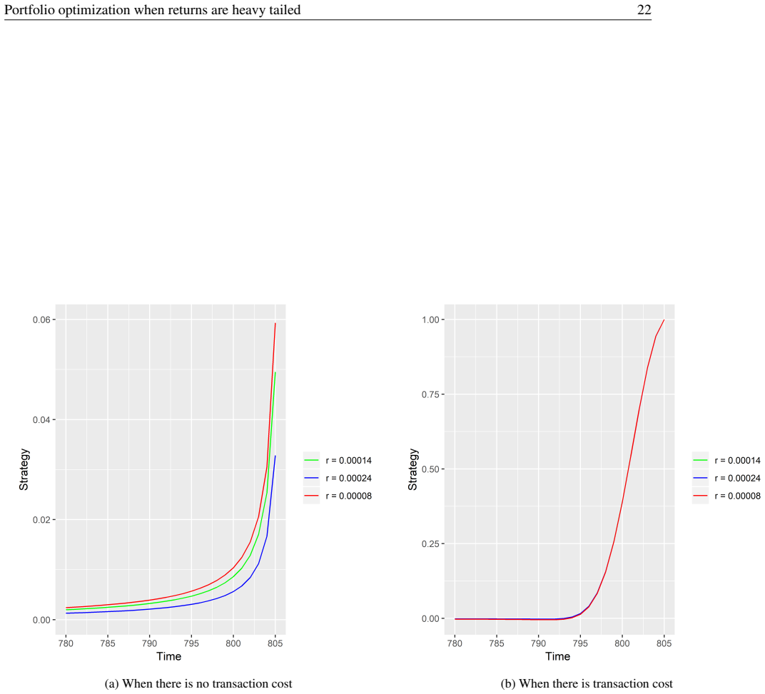
The central claim is that the Value-at-Risk constraint itself determines the optimal policy, and that dynamic programming then evaluates it. Starting from the wealth equation $L_t=\pi_t S_t+(1-\pi_t)r$, the authors require $P(L_{t-1}>Q_{0.05}\mid L_t>Q_{0.05})\ge 0.95$. For Pareto-distributed returns with scale $\lambda$ and tail index $\alpha$, substituting the survival function turns this into an integral inequality that solves to the recursion $\pi_{t-1}\le \pi_t(19.1977\pi_t+1)$ at a daily rate $r=0.00014$; the Weibull case gives $\pi_{t-1}\ge \pi_t(1-13.08\pi_t)$ and the Inverse Gaussian case an implicit relation solved numerically. With a 10% transaction cost the recursions become second-order. The value function is then obtained from the finite-horizon dynamic programming identity $u^\pi_{t-1}=(L_{t-1}-L_t)+E(u^\pi_t)$. In the non-parametric case the same conditional-probability constraint is evaluated by numerical integration against a kernel density estimate of the return distribution. The paper concludes that the resulting strategy tells the investor when to accumulate and when to liquidate the risky asset, and that transaction costs make the strategy nearly constant until the terminal period.
Load-bearing premise
The load-bearing premise is that the fitted heavy-tailed distribution is the true law of the daily returns, with the 5% VaR quantile used in the constraint lying inside the support of that distribution; if the quantile falls outside the support, the integral inequalities and recursions derived from them do not follow.
Editorial extensions
If this is right
- Under a fitted Pareto model, the next optimal holding is obtained directly from the current one by $\pi_{t-1}\le \pi_t(19.1977\pi_t+1)$, so the strategy is computable by hand, without Monte Carlo simulation.
- When the return distribution is unknown, the same VaR constraint solved by numerical integration against a kernel density estimate gives an implementable rule from historical data alone.
- With transaction costs, the recursion becomes second-order and the optimal policy is nearly flat until the horizon, predicting infrequent rebalancing followed by a sharp build-up or liquidation near the terminal date.
- The direction of the interest-rate effect matches standard intuition: lower bank rates push the optimal holding in the risky asset upward.
- Out-of-sample KS comparisons suggest the three two-parameter heavy-tailed candidates fit the data almost as well as the six-parameter mixture normal, so the approach controls tail risk at low estimation cost.
Reading between the lines
- A natural extension would replace the single 95% quantile condition with a family of quantiles or with expected shortfall, turning the one-path recursion into a full risk-return frontier.
- For multiple risky assets, the second moment may fail to exist, so a multi-asset version would need a rank-based or copula dependence measure in place of covariance; the paper flags this as future work, and the constraint-template approach suggests how to build it.
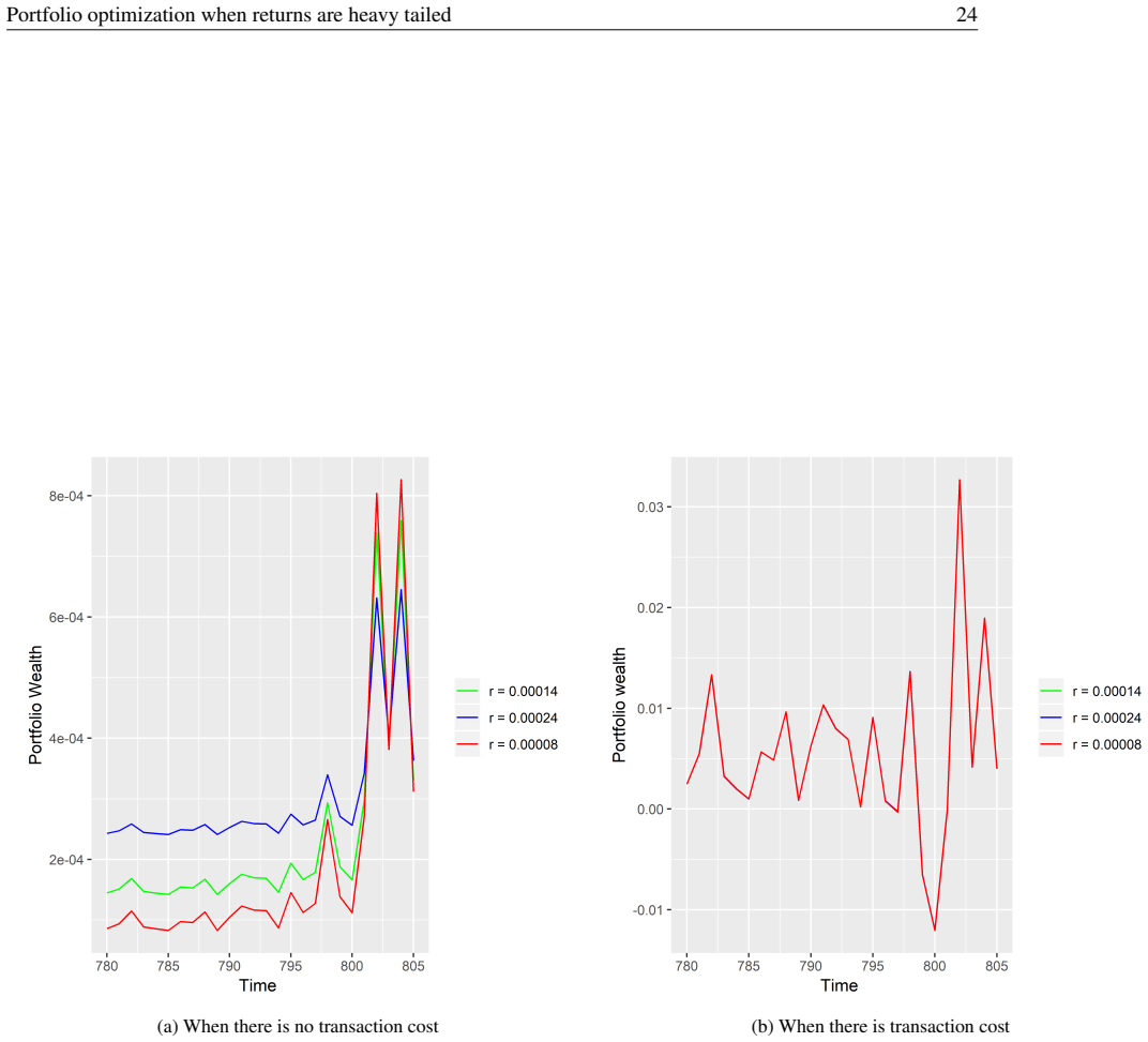
- In the kernel-density case, the value function and wealth fluctuate widely; smoothing or bandwidth regularization would likely be needed before using the recursion as a live trading rule.
- A holdout test could compare the realised frequency of wealth falling below the 5% quantile against the promised 5%: if the recursion is right, the violation rate should match the target over a long out-of-sample period.
Signed reviews
Editorial analysis
A structured set of objections, weighed in public.
Referee Report
Summary. The paper studies a discrete-time portfolio problem with one risky asset and a risk-free asset, where the investor maximizes expected utility (elsewhere, the 'median return') subject to a Value-at-Risk constraint, assuming heavy-tailed return distributions. The authors formulate the problem as a finite-horizon Markov decision process, derive backward recursions for the portfolio weight under Pareto, Weibull, and Inverse Gaussian return distributions, and also use a kernel density estimator for the unknown-distribution case. They calibrate the distributions to daily stock price data of Entergy Corporation, perform out-of-sample Kolmogorov-Smirnov tests, and numerically plot the implied optimal strategy, value function, and portfolio wealth with and without transaction costs. The central claims are that the recursions provide optimal strategies and that the value function is maximized at each time step.
Significance. If the claims were correct, the paper would offer a simple discrete-time rule for when to buy or liquidate a single risky asset under heavy-tailed returns while controlling VaR, with an explicit treatment of transaction costs. The empirical comparison of Pareto, Weibull, Inverse Gaussian, mixture-normal, and variance-gamma fits is a useful exercise, and the paper is transparent about its data source and KS-test methodology. However, the central optimality result is not established: the Bellman maximization in Eq. (2) is never carried out, the Pareto calibration is performed on stock prices rather than returns, the VaR quantile lies outside the fitted distribution's support, and the backward recursions are anchored on arbitrary terminal values. These are internal logical and empirical errors, not a matter of disagreement with current consensus. The paper's framework as presented does not support its stated conclusions, and the numerical outputs are not reliable.
major comments (4)
- [Section 2 and Section 3.1, Eqs. (2), (5), (6)] The Bellman optimality step is never performed. Equation (2) defines the optimal value function as a supremum over actions in the action space, but the recursive relation (6) is obtained solely by solving the VaR inequality (5) for π_{t-1} given π_t. No derivative is taken, no supremum or maximum over alternative actions is evaluated, and the reward W_{t-1}=L_{t-1}-L_t is only evaluated at a feasible point, not maximized. Consequently, the text's claim that these are 'optimal strategies' and that the value function is maximized is unsupported by the derivations. This is an internal gap: even if every distributional fit were correct, the paper would not have solved the optimization problem it states.
- [Section 3.1, Table 1 and Eq. (5)] The Pareto distribution is fitted to stock prices, not returns. The paper defines returns as (Price_t - Price_{t-1})/Price_{t-1}, but the estimated scale parameter λ = 85.34364 equals the minimum daily closing price of Entergy stock, and the estimated tail index α ≈ 10346 is implausible for return data. The quantile Q0.05 = 5×10^-6 λ ≈ 4.3×10^-4 lies far below the support of the fitted Pareto distribution (x ≥ λ = 85.34). As a result, the integral limits K_t in Eq. (5) are below the distribution's support, making the numerator and denominator of the constraint meaningless and the derived recursion (6) invalid. The same prices-versus-returns confusion affects the out-of-sample KS test, which validates the fit on prices rather than on the returns the model claims to address.
- [Section 3.1, Eq. (5)] The density used in Eq. (5) is not the density of the Pareto distribution defined earlier. The text defines the survival function as F(x) = (λ/x)^α for x ≥ λ, whose density is α λ^α / x^{α+1} on x ≥ λ. Equation (5), however, integrates α λ^α / (x+λ)^{α+1}, a shifted form with support x ≥ 0. This is an internal inconsistency, and the numerical value of the integral in Eq. (5) is therefore not a consequence of the stated Pareto model. The recursion (6) cannot be justified from the model as written.
- [Sections 3.2, 3.3, and 4.1] The backward recursions are anchored on arbitrary terminal strategy values that are assumed without justification: 0.00001 for Weibull, 0.1 for Inverse Gaussian, and 0.001 for the kernel-density case. These terminal values are not derived from the optimization problem or from any economic condition, yet they determine the entire path of the 'optimal' strategy through Eqs. (10), (13), and the KDE recursion. The dependence of the reported results on these externally imposed endpoints is not discussed, and it undermines the claim that the computed policies solve the stated maximization problem.
minor comments (5)
- [Abstract and Section 1.1] The abstract says the investor maximizes 'expected utility', while Section 1.1 says the investor seeks to 'maximize the median return of the portfolio'. These are different objectives, and the paper does not clarify which one is actually used in the MDP formulation.
- [Section 3.2, after Eq. (9)] The sentence 'Solving (8) and putting the values of λ and r = 0.00014...' should refer to Eq. (9), not Eq. (8), which is the transaction-cost recursion of the previous subsection.
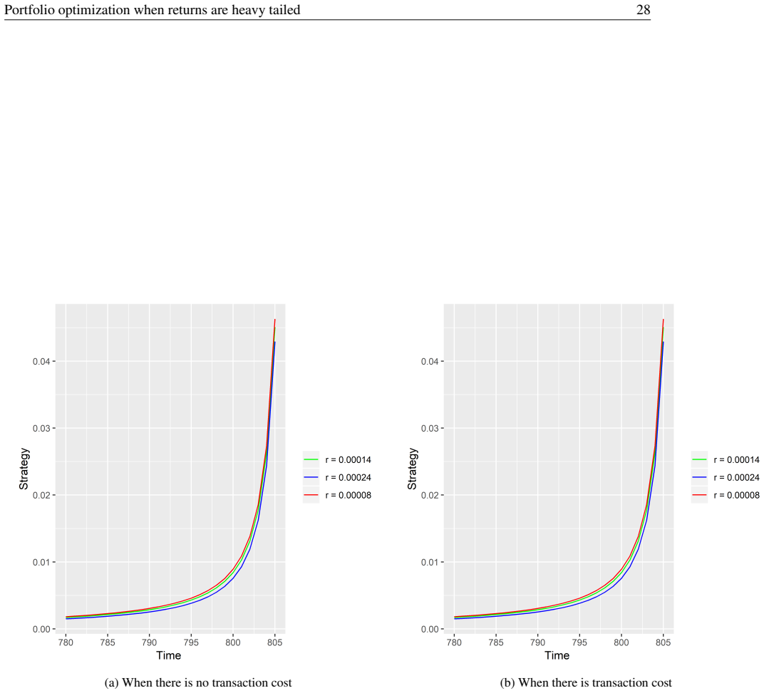
- [Figure captions 7-9] Figures 7-9 are described in the text as showing the Inverse Gaussian results, but the captions in the list of figures state 'considering Weibull distribution'. The captions should be corrected.
- [Table 6] The KS critical values reported in Table 6 are inconsistent: for a sample of size 50 the standard 5% critical value is about 0.192, but the table reports 0.12323 for the mixture normal and 0.156 for the variance gamma. The origin of these different critical values is not explained.
- [Section 4.1, Eq. (15)] In Eq. (15), the term F(0) appears without a clear definition of F; if F is the kernel CDF, then F(0) may not be meaningful for returns data that can take negative values. The expression should be stated more carefully.
Circularity Check
No circularity: the fitted distributions enter as model inputs and the policy is a constraint-derived object, not a fitted quantity renamed as a prediction; the serious issues are correctness gaps rather than circularity.
full rationale
The paper's derivation chain is not circular in the sense required here. The recursive policy relations (e.g., Eq. 6, Eq. 10, Eq. 13) are obtained by solving the VaR constraint equations (5), (9), and (13) after plugging in distribution parameters estimated from the data. The fitted parameters and quantiles are inputs to the optimization model, not outputs that are then claimed to be independent predictions of the same quantities. The policy is a deterministic function of the fitted distribution and the chosen terminal values, but that is true of any model-based decision rule and does not make the derivation equivalent to its inputs by construction. The KS tests are out-of-sample checks of the distributional fit only, and the paper does not present them as validating the strategy; this is a validation gap, not a self-referential reduction. The most serious defect is that the Bellman maximization in Eq. (2) is never actually carried out—the 'optimal' policies are merely feasible solutions of the VaR inequality—and the Pareto analysis appears to apply the fitted distribution outside its support. These are correctness and internal-validity failures, not circularity. No self-citation is load-bearing, and no known result is merely renamed. Under the quoted-reduction rule, no circular step is established.
Assumptions & free parameters
free parameters (15)
- Pareto scale lambda =
85.34364
- Pareto shape alpha =
10346.37374
- Weibull scale lambda =
1.2630
- Weibull shape alpha =
0.0104
- Inverse Gaussian mean mu =
0.0097
- Inverse Gaussian shape lambda =
0.0044
- Mixture normal parameters =
mu1=0.007286, mu2=0.02137, sigma=0.004741, pi=0.8646
- Variance gamma parameters =
c=0.005034, sigma=0.017160, theta=0.006051, nu=3.219203
- KDE bandwidth =
0.00271447
- Terminal strategy value for Weibull =
0.00001
- Terminal strategy value for Inverse Gaussian =
0.1
- Terminal value for KDE case =
0.001
- Transaction cost rate r1 =
10%
- Daily interest rates r =
0.00008, 0.00014, 0.00024
- VaR confidence level =
0.05
assumptions (6)
- ad hoc to paper The conditional probability constraint P(L_{t-1} > Q | L_t > Q) >= 0.95 is the correct formalization of VaR management.
- domain assumption The wealth equation L_t = pi_t S_t + (1-pi_t) r (with M=1) and the reward W_{t-1} = L_{t-1} - L_t define the investor's objective.
- domain assumption The stock price (or return) process is i.i.d. with the fitted parametric distribution, and this distribution provides the MDP transition probabilities.
- domain assumption The fitted distributions describe the data correctly; the KS test with 50 out-of-sample points is sufficient validation.
- domain assumption MLE parameter estimates are used as if they were the true parameters in the VaR constraint and recursions.
- ad hoc to paper The terminal optimal strategy values (0.00001, 0.1, 0.001) are given and the backward recursion is solved from these values.
Cite this review
Pith. "Pith review of Discrete time portfolio optimisation managing value at risk under heavy tail return distribution." pith.science (2026). https://pith.science/paper/7RPWGQVQ
@misc{pith2026190803907,
  author       = {Pith},
  title        = {Pith review of: Discrete time portfolio optimisation managing value at risk under heavy tail return distribution},
  year         = {2026},
  howpublished = {\url{https://pith.science/paper/7RPWGQVQ}},
  note         = {Machine review of arXiv:1908.03907}
}
read the original abstract
We consider an investor, whose portfolio consists of a single risky asset and a risk free asset, who wants to maximize his expected utility of the portfolio subject to the Value at Risk assuming a heavy tail distribution of the stock prices return. We use Markov Decision Process and dynamic programming principle to get the optimal strategies and the value function which maximize the expected utility for parametric as well as non parametric distributions. Due to lack of explicit solution in the non parametric case, we use numerical integration for optimization
Figures

Figures from the paper (9 more)




Reference graph
Works this paper leans on
-
[1]
The Econometrics of Financial Markets
John Y . Campbell, Andrew W. Lo, & A. Craig MacKinlay (1997), “The Econometrics of Financial Markets”, Princeton University Press
work page 1997
-
[2]
Martin L.Puterman (2005) Discrete stochastic dynamic programming, 79-82, Wiley
work page 2005
-
[3]
Miguel Ángel Martín Mato (2005) Classic and modern measures of risk in fixed-income portfolio optimization, The Journal of Risk Finance, V ol. 6 Issue: 5, 416-423
work page 2005
-
[4]
Fotios C. Harmantzis, Linyan Miao & Yifan Chien (2006) Empirical study of value-at-risk and expected short- fall models with heavy tails,The Journal of Risk Finance, V ol. 7 Issue: 2, pp.117-135
work page 2006
-
[5]
Young Shin Kim, Rosella Giacometti, Svetlozar T. Rachev, Frank J. Fabozzi & Domenico Mignacca (2012) Measuring financial risk and portfolio optimization with a non-Gaussian multivariate model, Annals of Opera- tions Research, V olume 201, Issue 1, pp 325–343
work page 2012
-
[6]
Grossman, S. J. & Zhou, Z. (1993) Optimal investment strategies for controlling drawdowns, Math. Finance 3(3), 241–276
work page 1993
- [7]
-
[8]
Paul A.Samuelson (1975) Lifetime portfolio selection by dynamic stochastic programming, Stochastic Opti- mization Models in Finance, Pages 517-524
work page 1975
Show all 26 references
-
[9]
Natalia Markovich (2007) Non parametric analysis of univariate heavy-tailed distribution,Wiley
2007
-
[10]
Lo (1998) Nonparametric Estimation of State-Price Densities Implicit in Financial Asset Prices, The Journal of Finance, 53 (2), 499 - 547
Yacine Aït-Sahalia & Andrew W. Lo (1998) Nonparametric Estimation of State-Price Densities Implicit in Financial Asset Prices, The Journal of Finance, 53 (2), 499 - 547
1998
-
[11]
Sukono, Pramono Sidi, Abdul Talib bin Bon & Sudradjat Supian (2017) Modeling of Mean-VaR portfolio optimization by risk tolerance when the utility function is quadratic, AIP Conference Proceedings 1827
2017
-
[12]
Lwin, Rong Qu & Bart L
Khin T. Lwin, Rong Qu & Bart L. MacCarthy (2017) Mean-VaR Portfolio Optimization: A Nonparametric Approach, EJOR, V olume 260(2), pp 751-766
2017
-
[13]
David Wozaba (2012) Value-at-Risk optimization using the difference of convex algorithm, OR Spectrum, V olume 34, Issue 4, pp 861–883
2012
-
[14]
Yinlam Chow & Mohammad Ghavamzadeh (2014) Algorithms for CVaR Optimization in MDPs, NIPS’14: Proceedings of the 27th International Conference on Neural Information Processing Systems, V olume 2, Pages 3509–3517 Portfolio optimization when returns are heavy tailed 18
2014
-
[15]
Bhatnagar, H
S. Bhatnagar, H. Prasad, & L.A. Prashanth (2013) Stochastic Recursive Algorithms for Optimization, volume
2013
-
[16]
Qian Chen & Richard H.Gerlach (2013) The two-sided Weibull distribution and forecasting financial tail risk, International Journal of Forecasting, volume 29 (4), 527-540
2013
-
[17]
Nicole Bauerle & Ulrich Rieder (2019) Markov Decision Processes Under Ambiguity, https://arxiv.org/abs/1907.02347
2019 arXiv
-
[18]
Lili Tang (2018) An actor-critic-based portfolio investment method inspired by benefit-risk optimization, Journal of Algorithms and Computational Technology, https://doi.org/10.1177/1748301818779059
2018 doi
-
[19]
Thomas W. Archibald & Edgar Possani (2019) Investment and operational decisions for start-up companies: a game theory and Markov decision process approach, Annals of Operations Research, https://doi.org/10.1007/s10479-019-03426-5
2019 doi
-
[20]
Yun-si Li, Ai-hua Li & Zhi-dong Liu (2018) Two Ways of Calculating VaR in Risk Management — An Empirical Study Based on CSI300 Index, Procedia Computer Science, V olume 139, Pages 432-439
2018
-
[21]
Daniel Evangelista Régisa & Rinaldo Artesa (2016) Using multi-state markov models to identify credit card risk, SciELO, V olume 26(2), http://dx.doi.org/10.1590/0103-6513.160814
2016
-
[22]
Yaqing Fu (2019) Variance Optimization for Continuous-Time Markov Decision Processes, Scientific Re- search Open Access, V olume 09(02),10.4236/ojs.2019.92014
2019
-
[23]
Iker Perez, David Hodge & Huiling Le (2016) Markov decision process algorithms for wealth allocation problems with defaultable bonds, Advances in Applied Probability, V olume 48(02), pp. 392-405
2016
-
[24]
https://www.quantopian.com, Accessed: 2018-10-10
2018
-
[25]
and Mikosch T
Embrechts P., Klüppelberg C. and Mikosch T. (1997) Modelling extremal events for insurance and finance. Berlin: Spring Verlag
1997
-
[26]
Kyprianou, A. E., W. Schoutens, and P. Wilmott (Eds.) (2005): Exotic option Pricing and Advanced L ´evy Models, Wiley. Portfolio optimization when returns are heavy tailed 19 List of Tables 1 Parameter Estimates of Pareto Distribution . . . . . . . . . . . . . . . . . . . . . ...
2005
Reviewed August 14, 2026 · model on record in the stance chip above.
Discussion (0). Continue with ORCID to comment.