REVIEW 2 major objections 6 minor 28 references
Mathematical and numerical study of a three-dimensional inverse eddy current problem
T0 review · 2 major / 6 minor · reviewed 2026-08-14 · deepseek-v4-flash
Pith's one-line read The inverse eddy current problem is ill-posed and non-unique, and the paper builds a regularized optimization that recovers inclusions numerically.
desk verdict The paper has solid compactness, regularity, and optimization work, but its headline non-uniqueness claim only proves non-uniqueness of the induced source, not of the conductivity itself. read the letter →
The pith
A machine-rendered reading of the paper's core claim, the machinery that carries it, and where it could break.
The reading
What carries the argument
The load-bearing object is the orthogonal decomposition of the secondary source space $L^2(\Omega_c)^3 = W \oplus W^\perp$, where $W$ consists of fields solving the homogeneous eddy-current equation inside the conductor with a vanishing tangential trace condition. Sources lying in $W^\perp$ are non-radiating: they produce $n\times E=0$ on the interface and measurement surface, so any source with a nonzero $W^\perp$ component is invisible to boundary data. The compactness of the forward map comes from the compact embedding $H^1(\Omega_c)\hookrightarrow L^2(\Omega_c)$ plus the continuity estimate linking conductivity differences to $H^{1/2}$ differences of the field in the air region, a regularity gain supplied by non-radiating-source arguments. Together these identify exactly why the inverse problem needs regularization.
What would settle it
A concrete test: pick two distinct admissible conductivities $\sigma_1,\sigma_2$ (for instance two different inclusions in $\Omega_c$), solve the forward problem (2.6) for each, and compare $n\times E(\sigma_1)$ and $n\times E(\sigma_2)$ on $\Gamma$. Exact equality would confirm true non-uniqueness of conductivity; a proof that $\sigma \mapsto \sigma E(\sigma)$ is injective on the admissible class would show only the source is ambiguous and leave conductivity uniqueness open.
Extended reading notes
Core claim
On the paper's own terms, the central discovery is that the inverse eddy current problem based on tangential electric boundary data is fundamentally ill-posed: the forward operator $\sigma \mapsto n\times E(\sigma)$ is compact from $H^1_0(\Omega_c)$ into $L^2(\Gamma)$, so bounded sets of conductivities produce precompact sets of data, and the secondary source $i\omega\sigma E(\sigma)$ is never uniquely determined when the measured field differs from the background field. The proof decomposes the source space as $L^2(\Omega_c)^3 = W \oplus W^\perp$; sources in $W^\perp$ are non-radiating (Theorem 3.1), and Theorem 3.2 shows both summands are nonzero, so the invisible component prevents unique recovery. The rest of the paper builds a well-posed surrogate: minimize $\Phi_\alpha(\sigma)=\frac12\|n\times(E(\sigma)-E_{\rm obs})\|^2_{L^2(\Gamma)}+\frac{\alpha}{2}\|\nabla\sigma\|^2_{L^2(\Omega_c)}$, prove existence and stability of its minimizers, and solve it numerically by a feasible Lagrangian, adjoint gradient, and NLCG with Sobolev gradient, with numerical reconstructions of separated inclusions.
Load-bearing premise
The reduction from conductivity to the secondary source $\sigma E(\sigma)$ is assumed lossless: Theorem 3.2 proves only that the source is not unique, and the paper takes that to mean the conductivity itself cannot be recovered, without exhibiting two distinct conductivities with identical boundary data.
Editorial extensions
If this is right
- Because the data-to-conductivity map is compact, small measurement errors can be amplified arbitrarily; any numerical inversion must be regularized, not just sampled finely.
- The non-radiating part of the induced source means perfect noise-free boundary data still cannot single out a unique conductivity distribution in general.
- The regularized functional has at least one minimizer and minimizers depend stably on the data, so the optimization formulation is a legitimate surrogate for the ill-posed inversion.
- The $H^{1/2}$ regularity of the field difference in the air region justifies using the computable $L^2(\Gamma)$ misfit instead of the harder $H^{-1/2}(\mathrm{Div};\Gamma)$ trace norm.
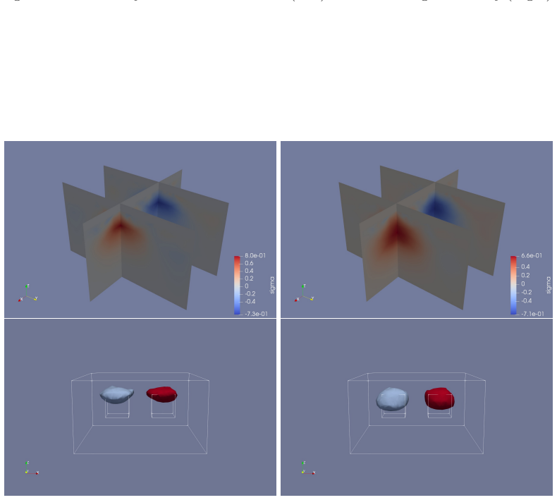
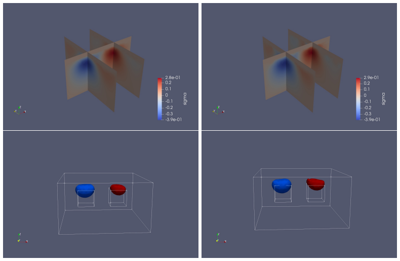
- The NLCG algorithm with the Sobolev gradient reconstructs locations and sizes of separated inclusions, and its convergence is markedly faster than with the plain $L^2$ gradient.
Reading between the lines
- The stated non-uniqueness is for the source $\sigma E(\sigma)$, not for $\sigma$ itself; whether two distinct conductivities can produce identical boundary data is left open, since the map $\sigma\mapsto \sigma E(\sigma)$ could conceivably be injective even though the source is not unique.
- The $W/W^\perp$ splitting suggests a natural definition of 'detectable' conductivity perturbations: a perturbation is invisible to first order if its secondary source lies mostly in $W^\perp$; this could be tested numerically by optimizing a perturbation to minimize the boundary trace.
- Because the splitting depends on frequency $\omega$, multi-frequency measurements may shrink the invisible component and could restore uniqueness even when single-frequency data cannot; this is an extension the paper does not pursue.
- The same Lagrangian/adjoint machinery would apply to recovering other parameters such as magnetic permeability or to multi-frequency data, since the structure of the state and adjoint systems is unchanged.
Signed reviews
Editorial analysis
A structured set of objections, weighed in public.
Referee Report
Summary. The paper studies the inverse eddy current problem of recovering the conductivity σ in a bounded three-dimensional conductor from tangential electric field measurements n×E on a boundary part Γ. The authors first prove well-posedness of the forward saddle-point formulation, establish a regularity result for E(σ)−Eobs in the air subdomain Ω0, and prove compactness of the map σ↦n×E(σ)|Γ. They then claim non-uniqueness of the conductivity recovery, formulate a Tikhonov-regularized constrained optimization problem, prove existence and stability of minimizers, derive the adjoint-based gradient, discretize the problem with edge elements, and propose a nonlinear conjugate gradient method with a Sobolev gradient. Numerical experiments on one and two inclusions are reported.
Significance. If the stated results are taken at face value, the paper contributes a fairly complete analysis pipeline for an eddy-current inversion problem: forward well-posedness, a regularity result that justifies using an L2 misfit on Γ, compactness of the forward map, existence/stability of regularized minimizers, and a concrete adjoint/NLCG algorithm with numerical demonstrations. The main advertised theoretical novelty, however, is the non-uniqueness of the conductivity recovery, and that claim is not established by the arguments in Section 3.2. The paper actually proves non-uniqueness of the equivalent source iωσE(σ) in the auxiliary inverse source problem, not non-uniqueness of σ itself. The optimization analysis and numerical framework are valuable and do not depend on the overclaimed conductivity non-uniqueness, so the paper is salvageable with a precise reformulation of the ill-posedness statement.
major comments (2)
- [§3.2, Theorem 3.2] Theorem 3.2 overreaches in a load-bearing way. The proof shows only that the secondary source Je = iωσE(σ) can be decomposed as J1 + J2 with J2 ∈ W⊥, J2 ≠ 0, and that by Theorem 3.1 the component J2 produces no tangential field on Γ. This means the inverse source problem (3.4) does not have a unique source. It does not produce two distinct conductivities σ and σ1 with n×E(σ) = n×E(σ1) on Γ. To obtain conductivity non-uniqueness one would need to construct σ1 ≠ σ such that iωσ1E(σ1) = J1 and n×E(σ1) = n×E(σ) on Γ, and one would need σ1 to be real-valued, nonnegative, compactly supported in Ωc, and in H1_0(Ωc). None of these properties is shown, and the fixed-point equation σ1 = J1/(iωE(σ1)) is not analyzed. Consequently the title of Section 3.2, the abstract's claim of non-uniqueness of the recovery process, and the concluding remarks overstate the result. The authors should either prove conductivity non-uniqueness or explicitly restrict the claim to non-uniqueness of the equivalent source in the inverse source problem.
- [§2.2, proof of Theorem 2.2] The proof of Theorem 2.2 contains a missing argument that is load-bearing for the regularity result. It is asserted that 'with the arguments in Theorem 3.1 of Section 3, we know that ∇φ is a non-radiating source, then Eφ|Ω0 = 0.' To apply the non-radiating criterion of Theorem 3.1, one needs to prove that ∇φ ∈ W⊥, where W is defined only later in Section 3.2. This is not shown in the proof, and it is not immediate from the displayed decomposition Je = J0 + ∇φ. A short argument using that every u ∈ W satisfies ∇·u = 0 in Ωc (from the equation in the definition of W) would close the gap, but as written the proof of Theorem 2.2 is incomplete. Since Theorem 2.2 is used to justify the L2 misfit functional and is subsequently invoked in Lemmas 2.3, 3.1, 3.2, and Theorem 3.3, this gap should be repaired explicitly.
minor comments (6)
- [Lemma 3.1] The statement says σn → σ* in L2(Γ), but the proof and the intended compactness argument require convergence in L2(Ωc); this should be corrected.
- [Lemma 3.2] The proof cites 'Lemma 2.2' for the regularity of E(σn)−E(σ*) in Ω0, but Lemma 2.2 is the uniqueness result; the regularity bound comes from Theorem 2.2 and Lemma 2.3. This citation should be fixed.
- [Theorem 2.1] The statement writes H1_Γ(Ωc) for the multiplier φ; the correct space is H1_Γ(Ω0) as used in the proof.
- [Theorem 3.2, proof] The phrase 'homogeneous eigenfunction corresponding to imaginary eigenvalue iωµσ0' is sign-inconsistent with the definition of W, which has +iωσ0u = 0; this should be corrected or clarified.
- [Remark 3.2] The expression Je = iωµσE(σ) is inconsistent with the earlier definition Je = iωσE(σ) in Section 3.2; the factor µ should be removed or the convention explained.
- [§5, Numerical experiments] The numerical section reports only visual comparisons and iteration counts; a quantitative reconstruction error with respect to the true σ and a clear stopping criterion would strengthen the feasibility claim.
Circularity Check
No significant circularity: the central compactness and non-uniqueness arguments are derived from the PDE and external theorems, not from the quantities they purport to establish.
full rationale
The main derivation chain is self-contained. The forward map from conductivity to n×E(σ)|Γ is defined by the eddy current equations, and compactness is proved via the compact embedding H1(Ωc) into L2(Ωc) together with the stability estimate of Section 2, not by assuming the conclusion. The non-uniqueness argument uses a non-radiating source decomposition of iωσE(σ) relative to the background field E0 and Theorem 3.1, which is proved by integration by parts and trace arguments; it does not define conductivity non-uniqueness into the theorem. The regularized optimization analysis uses standard compactness, weak lower semicontinuity, and adjoint-state calculations, with no parameter fitted to the boundary data and then renamed a prediction. Self-citations [7], [8], and [18] appear only for auxiliary coercivity sketches, discrete saddle-point well-posedness, and the Sobolev-gradient acceleration technique; none is load-bearing for the compactness, non-uniqueness, existence, or stability claims. The abstract's wording that non-uniqueness of the recovery process is established is broader than Theorem 3.2, which proves non-uniqueness only for σE(σ) and does not construct two distinct conductivities with identical boundary data; this is a logical gap or correctness risk, not a circular derivation. Therefore no circular step is present.
Assumptions & free parameters
free parameters (1)
- regularization parameter α =
10^-6 for clean data, 10^-4 for noisy data
assumptions (4)
- standard math H^1_0(Ωc) compactly embeds into L2(Ωc), and Lax-Milgram applies to the sesquilinear form a(·,·).
- domain assumption Domain geometry: Ω is convex polyhedral, Ω0 and Ωc are simply-connected polyhedra, Γ0c is Lipschitz polyhedral; σ0 is constant in Ωc; Js is compactly supported in Ω0 with ∇·Js=0.
- domain assumption Regularity imbedding XN(Ω0) ⊂ H^s(Ω0) for some s>1/2, imported from Theorem 6.1 of [12].
- domain assumption The observed data Eobs are generated by the same model with a true conductivity σ0+σe.
Cite this review
Pith. "Pith review of Mathematical and numerical study of a three-dimensional inverse eddy current problem." pith.science (2026). https://pith.science/paper/7STTWHXB
@misc{pith2026190808683,
  author       = {Pith},
  title        = {Pith review of: Mathematical and numerical study of a three-dimensional inverse eddy current problem},
  year         = {2026},
  howpublished = {\url{https://pith.science/paper/7STTWHXB}},
  note         = {Machine review of arXiv:1908.08683}
}
read the original abstract
We study an inverse problem associated with an eddy current model. We first address the ill-posedness of the inverse problem by proving the compactness of the forward map with respect to the conductivity and the non-uniqueness of the recovery process. Then by virtue of non-radiating source conceptions, we establish a regularity result for the tangential trace of the true solution on the boundary, which is necessary to justify our subsequent mathematical formulation. After that, we formulate the inverse problem as a constrained optimization problem with an appropriate regularization and prove the existence and stability of the regularized minimizers. To facilitate the numerical solution of the nonlinear non-convex constrained optimization, we introduce a feasible Lagrangian and its discrete variant. Then the gradient of the objective functional is derived using the adjoint technique. By means of the gradient, a nonlinear conjugate gradient method is formulated for solving the optimization system, and a Sobolev gradient is incorporated to accelerate the iterative process. Numerical examples are provided to demonstrate the feasibility of the proposed algorithm.
Figures

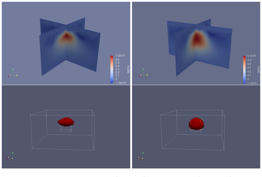

Figures from the paper (2 more)
Reference graph
Works this paper leans on
-
[26]
A. Rodriguez, J. Camano and A. Valli, Inverse source problems for eddy current equations, Inverse Probl., 28(2012), 015006
work page 2012
-
[12]
M. Costabel, M. Dauge and S. Nicaise, Singularities of eddy current problems, ESAIM: M2AN, 37(2003), 807-831
work page 2003
-
[10]
Z. Chen and J. Zou, An augmented lagrangian method for identifying discontinuous parameters in elliptic systems, SIAM, J. Control Optim., 37(1999), 892-910
work page 1999
-
[7]
J. Chen, Z. Chen, T. Cui and L.-B. Zhang, An adaptive finite method for the eddy current model with circuit/field coupings, SIAM J. Sci. Comput., 32(2010), 1020-1042
work page 2010
-
[8]
J. Chen, Y. Xu, and J. Zou, An Adaptive Edge Element Method and Its Convergence for a Saddle-Point Problem from Magnetostatics, Numer. Meth. Part. D. E., 28(2012), 1643-1666
work page 2012
-
[18]
B. Jin, J. Zou, Numerical estimation of Robin coefficient in a stationary diffusion equation, IMA J. Numer. Anal., 30(2010), 677-701
work page 2010
- [1]
- [2]
Show all 28 references
-
[3]
Ammari, J
H. Ammari, J. Chen, Z. Chen, D. Volkov and H. Wang, Detection and classification from electromagnetic induction data, J. Comput. Phys., 301 (2015), 201-217 20
2015
-
[4]
Amrouche, C
C. Amrouche, C. Bernardi, M. Dauge, and V. Girault, Vector potentials in three-dimensional nonsmooth domains, Math. Methods Appl. Sci., 21 (1998), 823-864
1998
-
[5]
Badia and T
A. Badia and T. Nara, Inverse dipole source problem for time-harmonic Maxwell equations: algebraic algorithm and H¨ older stability, Inverse Probl., 29 (2013), 015007 (19pp)
2013
-
[6]
A. Buffa, M. Costabel, D. Sheen, On traces for H(curl, Ω) in Lipschitz domains, J. Math. Anal. Appl., 276 (2002), 845-867
2002
-
[9]
Z. Chen, W. Wang and W. Zheng, An adaptive multilevel method for time-harmonic Maxwell equation with singularities, SIAM J. Sci. Comput., 29(2007), 118-138
2007
-
[11]
P. G. Ciarlet, Linear and nonlinear functioanl analysis with applications, SIAM, Philadelphia, 2013
2013
-
[13]
H. Feng, D. Jiang and J. Zou, Simultaneous identification of electric permittivity and magnetic permeability, Inverse Probl., 26(2010), 095009(20pp)
2010
-
[14]
X. Feng, S. Lenhart, V. Protopopescu, L. Rachele and B. Sutton, Identification problem for the wave equation with Neumann data input and Dirichlet data observations, Nonlinear Anal. 52(2003), 1777-1795
2003
-
[15]
Haber, Computational methods in geophysical electromagnetics, 2015, SIAM
E. Haber, Computational methods in geophysical electromagnetics, 2015, SIAM
2015
-
[16]
Hiptmair and J
R. Hiptmair and J. Xu, Nodal auxiliary space preconditioning in H(curl) and H(div) spaces, SIAM J. Numer. Anal., 45 (2007), 2483-2509
2007
-
[17]
Jackson, Classical electrodynamics, 3rd edition, Wiley, 1999
J.D. Jackson, Classical electrodynamics, 3rd edition, Wiley, 1999
1999
-
[19]
Li and W
P. Li and W. Zheng, An H−ψ formulation for the three-dimensional eddy current problem in laminated structures, J. Differential Equations, 254 (2013), 3476-3500
2013
-
[20]
Monk, Finite element methods for Maxwell’s equations, Oxford University Press, 2003
P. Monk, Finite element methods for Maxwell’s equations, Oxford University Press, 2003
2003
-
[21]
Norton, J.R
S.J. Norton, J.R. Bowler, Theory of eddy current inversion, J. Appl. Phys., 73(1993), 501-512
1993
-
[22]
A. J. Peyton, Electromagnetic induction tomography. Industrial Tomography, Woodhead Publishing, (2015), 61-107
2015
-
[23]
Parallel Hierarchical grid, available at http://lsec.cc.ac.cn/phg/
PHG. Parallel Hierarchical grid, available at http://lsec.cc.ac.cn/phg/
-
[24]
Pratt, C
R. Pratt, C. Shin and G. Hicks, Gauss-Newton and full Newton methods in frequency-space seismic wave- form inversion, Geophys. J. Int., 133(1998), 341-362
1998
-
[25]
Dos Reis, M
D. Dos Reis, M. Lambert and D. Lesselier, Eddy-current evaluation of three-dimensional defects in a metal plate, Inverse Probl., 18(2002), 1857-1871
2002
-
[27]
Rodriguez, A
A. Rodriguez, A. Valli, Eddy Current Approximation of Maxwell Equations, Springer 2010
2010
-
[28]
M. S. Zhdanov, Inverse theory and applications in geophysics, 2nd Edition, 2015, Elsevier 21
2015
Reviewed August 14, 2026 · model on record in the stance chip above.
Discussion (0). Continue with ORCID to comment.