REVIEW 4 major objections 4 minor 59 references
The Cooling of Old White Dwarfs in 47 Tucanae
T0 review · 4 major / 4 minor · reviewed 2026-08-06 · deepseek-v4-flash
Pith's one-line read Deep Hubble data on 47 Tuc's oldest white dwarfs favour a hydrogen envelope of q_H = 2.82e-4 and a 0.5314 solar-mass white dwarf, with standard MESA diffusion reproducing the luminosity function.
desk verdict Careful first statistical fit of old WD cooling in 47 Tuc; the thick-envelope preference is real but sits at the grid edge and the F814W pass is weaker than the paper lets on. read the letter →
The pith
A machine-rendered reading of the paper's core claim, the machinery that carries it, and where it could break.
The reading
What carries the argument
The load-bearing quantity is the hydrogen-envelope thickness $q_H = M_H/M_{\rm WD}$, defined at a reference cooling time of 10 Myr, because it controls the convective-coupling bump in the cooling curve at exactly the late times and faint magnitudes the deep data probe. The argument runs on three linked components: a grid of MESA white-dwarf cooling models varying mass ($0.5092$-$0.5535\,M_\odot$), $q_H$ ($\log_{10} q_H = -3.55$ to $-3.95$), and diffusion treatment (standard ideal-gas Burgers diffusion; a custom version that multiplies the concentration-diffusion term by $1/(1+(\Gamma_k/A)^B)$ with $A=0.0625$, $B=1$, calibrated against small molecular-dynamics simulations of H-He plasmas; and no diffusion); an unbinned likelihood that folds in artificial-stars photometric error distributions, a proper-motion completeness correction, and a Gaussian birthrate prior from Gaia EDR3 red giants; and pure-hydrogen (DA) bolometric corrections that move the models into HST F606W/F814W magnitude space.
What would settle it
Take spectra, or narrow-band colours that separate H from He atmospheres, for the faintest members of this same 47 Tuc cooling sequence (F606W near 28). If a substantial fraction, on the order of ten percent, turn out to be helium-atmosphere white dwarfs or unresolved binaries, their colour-magnitude positions would not follow the DA bolometric corrections, and the recovered $\log_{10} q_H = -3.55$ and $M_{\rm WD} = 0.5314\,M_\odot$ would be biased; if they are overwhelmingly single DA stars, the interpretation stands. A computational version of the same test: refit the identical likelihood machinery to a luminosity function with essentially perfect faint-end completeness; either the standard-diffusion versus modified-diffusion degeneracy resolves itself, which would confirm the constraint is genuinely about envelope thickness, or it persists, which would show the data cannot separate the two effects.
Extended reading notes
Core claim
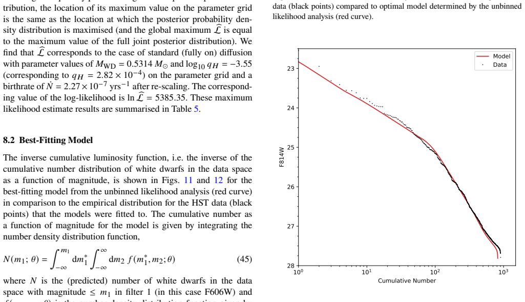
The central claim is that the standard MESA implementation of element diffusion, which solves Burgers' diffusion equations under an ideal-gas approximation for the ions, produces white-dwarf cooling models that reproduce the cumulative luminosity function of 47 Tuc's oldest white dwarfs, provided the hydrogen envelope is thick. On the model grid spanning masses 0.5092 to 0.5535 solar masses and envelope thicknesses $\log_{10} q_H$ from $-3.95$ to $-3.55$, the maximum-likelihood model has $q_H = 2.82\times 10^{-4}$, $M_{\rm WD} = 0.5314\,M_\odot$, and a birthrate of $2.27\times 10^{-7}\,\mathrm{yr^{-1}}$ that sits 1.5$\sigma$ from the independent red-giant-derived prior. The authors locate the physical leverage in the luminosity bump produced when the outer convection zone breaks through to the degenerate core, the convective-coupling feature whose size Tassoul et al. (1990) showed depends sensitively on H-envelope thickness, which coincides with the onset of core crystallisation and falls exactly where the faint-end data are most numerous. They also state that a modified diffusion treatment that suppresses concentration diffusion at the H/He boundary, fitted with somewhat thinner envelopes, is comparably likely and cannot be distinguished at a statistically significant level, while no-diffusion models fall outside the 2$\sigma$ contour; they conclude that the data favour thicker H envelopes but leave a partial degeneracy between envelope thickness and the diffusion prescription (Sections 8-9). The paper itself flags that faint-end completeness is the limiting factor and that this degeneracy is the reason the analysis has reached the limit of what this data set can say (Section 10).
Load-bearing premise
The load-bearing premise is that every faint white dwarf in the cleaned sample is a single hydrogen-atmosphere (DA) white dwarf: the model grid contains only pure-hydrogen envelopes and the bolometric corrections are for DA stars (Section 7), so a substantial helium-atmosphere or unresolved-binary population would bias the inferred envelope thickness and mass.
Editorial extensions
If this is right
- The typical old white dwarf in 47 Tuc is inferred to have a thick hydrogen envelope, $\log_{10} q_H \approx -3.55$, a mass near $0.5314\,M_\odot$, and a birthrate of $2.27\times 10^{-7}\,\mathrm{yr^{-1}}$, consistent with the cluster's red-giant supply.
- MESA's standard diffusion treatment, with its ideal-gas approximation for ions, is adequate for modelling white-dwarf cooling through convective coupling and into core crystallisation, the regime tested here.
- The data cannot statistically separate envelope thickness from the diffusion prescription: standard diffusion with thicker envelopes and non-ideal-gas-suppressed diffusion with somewhat thinner envelopes are similarly likely, so neither parameter alone is pinned down.
- Models with diffusion switched off are disfavoured at more than 2$\sigma$, so some diffusion is required to reproduce the shape of the observed luminosity function.
- The faint end of the cooling sequence is what carries the constraint: truncating the data space at brighter magnitudes (F606W $\leq 28.25$) reverses the preference toward no diffusion with thinner envelopes.
Reading between the lines
- If thick hydrogen envelopes are the norm for old cluster white dwarfs, white-dwarf cooling ages used to date globular clusters would shift relative to models with thinner envelopes, because a thicker envelope delays the convective-coupling bump; the paper does not draw this cosmochronology consequence.
- The recovered $q_H$ and mass are averages over a population assumed to be all single hydrogen-atmosphere (DA) white dwarfs; a spectroscopic census of the faintest cooling-sequence members in this field would show whether a helium-atmosphere or binary fraction is biasing the envelope measurement.
- The same grid-and-likelihood machinery applied to a second old globular cluster with comparably deep photometry would test whether the inferred envelope thickness is a universal property of old white dwarfs or is specific to 47 Tuc.
- The non-ideal diffusion suppression used here is a fiducial prescription; if the true suppression of concentration diffusion in the liquid core is stronger, the same luminosity function could be reproduced with thinner envelopes, so the reported $q_H$ should be read jointly with the diffusion assumption rather than as an isolated measurement.
Editorial analysis
A structured set of objections, weighed in public.
Referee Report
Summary. The paper analyzes deep HST ACS/WFC observations of the globular cluster 47 Tucanae and constructs a suite of MESA white dwarf cooling models with varying white dwarf mass, H-envelope thickness, and treatment of element diffusion (standard MESA, a custom non-ideal correction, and no diffusion). An unbinned Poisson likelihood, including photometric completeness and proper-motion cleaning, is used to compare the models to the observed CMD. The best-fitting model uses standard MESA diffusion with M_WD = 0.5314 Msun, log10 q_H = -3.55, and a birthrate of 2.27e-7 yr^-1, and the authors conclude that thicker H envelopes are preferred and that the standard MESA diffusion treatment reproduces the cumulative white dwarf luminosity function well into the convective-coupling and crystallisation regime.
Significance. The paper brings a careful, statistically explicit treatment to an important dataset: the proper-motion cleaning and SMC contamination calibration are documented, the completeness is propagated through the likelihood in Eq. (30), and the analytic birthrate rescaling is a clean way to reduce the parameter space. If the central result holds, it provides a useful constraint on H-envelope thickness in an old globular cluster and supports the adequacy of MESA's ideal-gas diffusion treatment to late cooling times. The authors are also honest about the degeneracy between diffusion treatment and envelope thickness. However, the central inference is conditional on the sample being essentially all single DA white dwarfs, and the reported significance is weakened by a post-hoc data-space choice and a best fit that lies at the edge of the model grid.
major comments (4)
- [Section 7, Eq. (38)] The likelihood treats every observed object as a single DA white dwarf: the model grid in Section 5.2 contains only pure-H envelopes and Section 7 adopts DA bolometric corrections. A non-trivial population of He-atmosphere (DB/DC) white dwarfs or unresolved binaries would have different colours and cooling rates and would bias the inferred q_H and the diffusion preference. The paper neither justifies the single-DA assumption for 47 Tuc's old white dwarfs nor tests it. Please add a two-population mixture fit, or use external constraints on the DA fraction, or at minimum quantify how a plausible He-atmosphere or binary fraction would shift the best-fit q_H and mass.
- [Section 7, data-space cutoff] The authors state that multiple cut-offs between F606W = 28.0 and 29.0 were tested and that 28.5 was chosen because it 'optimised this trade-off'. Because the data space is selected using the same data that are subsequently fit, the likelihood comparison and the KS p-values in Table 6 do not account for this post-hoc selection. The reported preference and significance are therefore conditional on a choice made after inspecting the data. Please report results for all tested cut-offs, or use a validation/hold-out procedure, or otherwise correct the significance statement.
- [Section 8.1, Table 5] The best fit lies at the thickest grid value log10 q_H = -3.55, so the conclusion that 'thicker H envelopes are preferred' is a boundary result unless -3.55 is demonstrated to be at the physical upper limit described in Section 5.2. The paper should state explicitly whether this grid value is the physical maximum, and if not, extend the grid to thicker envelopes or show the likelihood profile beyond -3.55; otherwise the preferred value is not a genuine interior maximum of the likelihood.
- [Table 6] The F814W marginal KS p-value is 0.041, which would be rejected at the conventional 5% level, yet the text calls the p-values 'large' and applies a threshold of 10^-4. This overstates the goodness of fit. The authors should either report these p-values as marginal and discuss the implied tension, or apply a more appropriate goodness-of-fit statistic (e.g., a full two-dimensional or Anderson-Darling test).
minor comments (4)
- [Section 5.2] The white dwarf mass is given as 0.5338 Msun here but as 0.5388 Msun in Section 5.1 and elsewhere; one of these is a typo and should be corrected.
- [Section 6] The text says the birthrate models use 'initial_z of 4e-4', while Section 5.1 sets initial_z = 4.0e-3; the value 4e-4 appears to be a typo and should be corrected.
- [Figures 9 and 10] The filled contours are described as not being credible regions, which is appropriate, but the figure captions should state more prominently that the plotted contours are probability-density levels, not enclosed-probability regions, to avoid misinterpretation.
- [Section 9] The statement that the modified-diffusion parameters are fixed at fiducial values is useful, but a short discussion of how the fiducial choice and its uncertainty might affect the comparison between standard and modified diffusion would strengthen the interpretation.
Circularity Check
No significant circularity: the cooling-model grid is fitted to the observed CMD, and the cited prior works are used as data, method, or ancillary inputs rather than to force the central inference.
full rationale
The paper's derivation chain is self-contained. A grid of MESA white-dwarf cooling models is constructed by varying M_WD, H-envelope thickness q_H, and diffusion treatment, and an unbinned likelihood (Eq. 38) is used to compare these models to the observed 47 Tuc photometry. The best-fitting parameters (M_WD = 0.5314 Msun, log10 q_H = -3.55, standard diffusion) are genuinely estimated from the data; no equation defines q_H or the diffusion preference in terms of the observed luminosity function, and no fitted parameter is relabelled as an out-of-sample prediction. The 'test' of MESA diffusion is an in-sample model comparison, but it is not forced by construction: the grid uses discrete parameter values and the KS p-values (0.077 for F606W, 0.041 for F814W) show the match is not exact. Citations to Obertas et al. (2018), Goldsbury et al. (2016), Heyl et al. (2015), and Chen et al. (2018) are used for the data set, the likelihood method, the initial-mass-loss prescription, and the cluster distance, respectively; none of these carries the burden of proving that standard diffusion is adequate or that thick envelopes are preferred. The DA-only atmospheric assumption and the edge-of-grid preference for the thickest envelope are modeling limitations, not circular steps.
Assumptions & free parameters
free parameters (5)
- White dwarf mass M_WD =
0.5314 M_sun (grid best-fit)
- H envelope thickness log10 q_H =
-3.55 (q_H = 2.82e-4)
- White dwarf birthrate =
2.27e-7 yr^-1
- Modified diffusion parameters A and B =
A = 0.0625, B = 1
- f_CR piecewise linear parameters =
F606W0 = 27.00, f_CR,0 = 0.9158, a1 = -0.0060, a2 = -0.1297
assumptions (6)
- domain assumption MESA stellar evolution code accurately simulates white dwarf cooling for the modeled parameter range.
- domain assumption Photometric error distribution E is independent of position in the field.
- domain assumption Number density and error distribution are uniform across the HST field, so the likelihood does not depend on radius.
- domain assumption All target white dwarfs are DA (hydrogen-atmosphere) stars.
- domain assumption The distance d = 4.45 kpc and reddening E(B-V) = 0.04 are correct.
- ad hoc to paper MESA's standard diffusion ideal-gas approximation is a reasonable baseline; the custom correction is ad hoc.
Cite this review
Pith. "Pith review of The Cooling of Old White Dwarfs in 47 Tucanae." pith.science (2026). https://pith.science/paper/7XOERFHD
@misc{pith2026250722046,
  author       = {Pith},
  title        = {Pith review of: The Cooling of Old White Dwarfs in 47 Tucanae},
  year         = {2026},
  howpublished = {\url{https://pith.science/paper/7XOERFHD}},
  note         = {Machine review of arXiv:2507.22046}
}
read the original abstract
We analyse the cooling of white dwarfs in the globular cluster 47 Tucanae (47 Tuc) using deep observations from the {\it Hubble Space Telescope} that resolve the white dwarf cooling sequence to late enough cooling times that the envelope has become convectively coupled to the core. At these late times, the thickness of the outer H envelope is an important consideration in modelling the cooling. Using the stellar evolution software Modules for Experiments in Stellar Astrophysics, we create a suite of white dwarf cooling models for different thicknesses of the H envelope and different white dwarf masses. An unbinned likelihood analysis is performed to compare the cooling models to the observations in order to constrain the values of these key parameters. We find that thicker H envelopes are preferred, with the best-fitting models reproducing the observed cumulative 47 Tuc white dwarf luminosity functions well.
Figures


Figures from the paper (8 more)


Reference graph
Works this paper leans on
-
[1]
Atmospheres from very low-mass stars to extrasolar planets
Allard F., Homeier D., Freytag B., Sharp C. M., 2012, in Reyl \'e C., Charbonnel C., Schultheis M., eds, EAS Publications Series Vol. 57, EAS Publications Series. pp 3--43 ( @eprint arXiv 1206.1021 ), @doi 10.1051/eas/1257001
work page Pith review arXiv 2012
-
[2]
Aringer B., Girardi L., Nowotny W., Marigo P., Lederer M. T., 2009, @doi [ ] 10.1051/0004-6361/200911703 , https://ui.adsabs.harvard.edu/abs/2009A&A...503..913A 503, 913
-
[3]
Aringer B., Girardi L., Nowotny W., Marigo P., Bressan A., 2016, @doi [ ] 10.1093/mnras/stw222 , https://ui.adsabs.harvard.edu/abs/2016MNRAS.457.3611A 457, 3611
-
[4]
B \'e dard A., Bergeron P., Brassard P., Fontaine G., 2020, @doi [ ] 10.3847/1538-4357/abafbe , https://ui.adsabs.harvard.edu/abs/2020ApJ...901...93B 901, 93
-
[5]
Bergeron P., Wesemael F., Beauchamp A., 1995, @doi [ ] 10.1086/133661 , https://ui.adsabs.harvard.edu/abs/1995PASP..107.1047B 107, 1047
doi:10.1086/133661 1995
-
[6]
Bjork S. R., Chaboyer B., 2006, @doi [ ] 10.1086/500505 , https://ui.adsabs.harvard.edu/abs/2006ApJ...641.1102B 641, 1102
-
[7]
Bloecker T., 1995, , https://ui.adsabs.harvard.edu/abs/1995A&A...297..727B 297, 727
work page 1995
-
[8]
Blouin S., Dufour P., Allard N. F., 2018, @doi [ ] 10.3847/1538-4357/aad4a9 , https://ui.adsabs.harvard.edu/abs/2018ApJ...863..184B 863, 184
Show all 59 references
-
[9]
B \"o hm K.-H., 1968, @doi [ ] 10.1007/BF00650915 , https://ui.adsabs.harvard.edu/abs/1968Ap&SS...2..375B 2, 375
1968 doi
-
[10]
Bressan A., Marigo P., Girardi L., Salasnich B., Dal Cero C., Rubele S., Nanni A., 2012, @doi [ ] 10.1111/j.1365-2966.2012.21948.x , https://ui.adsabs.harvard.edu/abs/2012MNRAS.427..127B 427, 127
2012
-
[11]
M., 1969, Flow Equations for Composite Gases
Burgers J. M., 1969, Flow Equations for Composite Gases . Academic Press, Inc., New York
1969
-
[12]
A., Clayton G
Cardelli J. A., Clayton G. C., Mathis J. S., 1989, @doi [ ] 10.1086/167900 , https://ui.adsabs.harvard.edu/abs/1989ApJ...345..245C 345, 245
1989 doi
-
[13]
Cassisi S., Mar \' n-Franch A., Salaris M., Aparicio A., Monelli M., Pietrinferni A., 2011, @doi [ ] 10.1051/0004-6361/201016066 , https://ui.adsabs.harvard.edu/abs/2011A&A...527A..59C 527, A59
2011 doi
- [14]
-
[15]
Chen Y., Bressan A., Girardi L., Marigo P., Kong X., Lanza A., 2015, @doi [ ] 10.1093/mnras/stv1281 , https://ui.adsabs.harvard.edu/abs/2015MNRAS.452.1068C 452, 1068
2015 doi
-
[16]
Chen S., Richer H., Caiazzo I., Heyl J., 2018, @doi [ ] 10.3847/1538-4357/aae089 , https://ui.adsabs.harvard.edu/abs/2018ApJ...867..132C 867, 132
2018 doi
-
[17]
Chen Y., et al., 2019, @doi [ ] 10.1051/0004-6361/201936612 , https://ui.adsabs.harvard.edu/abs/2019A&A...632A.105C 632, A105
2019 doi
-
[18]
Christensen-Dalsgaard J., 2015, @doi [ ] 10.1093/mnras/stv1656 , https://ui.adsabs.harvard.edu/abs/2015MNRAS.453..666C 453, 666
2015 doi
-
[19]
Di Cecco A., et al., 2010, @doi [ ] 10.1088/0004-637X/712/1/527 , https://ui.adsabs.harvard.edu/abs/2010ApJ...712..527D 712, 527
2010 doi
-
[20]
Ferraro F. R., Lapenna E., Mucciarelli A., Lanzoni B., Dalessandro E., Pallanca C., Massari D., 2016, @doi [ ] 10.3847/0004-637X/816/2/70 , https://ui.adsabs.harvard.edu/abs/2016ApJ...816...70F 816, 70
2016 doi
-
[21]
Fontaine G., Brassard P., Bergeron P., 2001, @doi [ ] 10.1086/319535 , https://ui.adsabs.harvard.edu/abs/2001PASP..113..409F 113, 409
2001 doi
-
[22]
Fu X., Bressan A., Marigo P., Girardi L., Montalb \'a n J., Chen Y., Nanni A., 2018, @doi [ ] 10.1093/mnras/sty235 , https://ui.adsabs.harvard.edu/abs/2018MNRAS.476..496F 476, 496
2018 doi
-
[23]
B., Anderson J., Dotter A., Sarajedini A., Woodley K., 2010, @doi [ ] 10.1088/0004-6256/140/6/1830 , https://ui.adsabs.harvard.edu/abs/2010AJ....140.1830G 140, 1830
Goldsbury R., Richer H. B., Anderson J., Dotter A., Sarajedini A., Woodley K., 2010, @doi [ ] 10.1088/0004-6256/140/6/1830 , https://ui.adsabs.harvard.edu/abs/2010AJ....140.1830G 140, 1830
2010 doi
-
[24]
B., Kalirai J
Goldsbury R., Heyl J., Richer H. B., Kalirai J. S., Tremblay P. E., 2016, @doi [ ] 10.3847/0004-637X/821/1/27 , https://ui.adsabs.harvard.edu/abs/2016ApJ...821...27G 821, 27
2016 doi
-
[25]
Hansen B. M. S., et al., 2013, @doi [ ] 10.1038/nature12334 , https://ui.adsabs.harvard.edu/abs/2013Natur.500...51H 500, 51
2013 doi
-
[26]
H., Grebel E
Harbeck D., Smith G. H., Grebel E. K., 2003, @doi [ ] 10.1086/345570 , https://ui.adsabs.harvard.edu/abs/2003AJ....125..197H 125, 197
2003 doi
-
[27]
E., 1996, @doi [ ] 10.1086/118116 , https://ui.adsabs.harvard.edu/abs/1996AJ....112.1487H 112, 1487
Harris W. E., 1996, @doi [ ] 10.1086/118116 , https://ui.adsabs.harvard.edu/abs/1996AJ....112.1487H 112, 1487
1996 doi
-
[28]
B., Marigo P., Antolini E., Goldsbury R., Parada J., 2015, @doi [ ] 10.1088/0004-637X/810/2/127 , https://ui.adsabs.harvard.edu/abs/2015ApJ...810..127H 810, 127
Heyl J., Kalirai J., Richer H. B., Marigo P., Antolini E., Goldsbury R., Parada J., 2015, @doi [ ] 10.1088/0004-637X/810/2/127 , https://ui.adsabs.harvard.edu/abs/2015ApJ...810..127H 810, 127
2015 doi
-
[29]
B., Bergeron P., 2006, @doi [ ] 10.1086/505938 , https://ui.adsabs.harvard.edu/abs/2006AJ....132.1221H 132, 1221
Holberg J. B., Bergeron P., 2006, @doi [ ] 10.1086/505938 , https://ui.adsabs.harvard.edu/abs/2006AJ....132.1221H 132, 1221
2006 doi
-
[30]
J., MacDonald J., 1985, @doi [ ] 10.1086/163473 , https://ui.adsabs.harvard.edu/abs/1985ApJ...296..540I 296, 540
Iben I. J., MacDonald J., 1985, @doi [ ] 10.1086/163473 , https://ui.adsabs.harvard.edu/abs/1985ApJ...296..540I 296, 540
1985 doi
-
[31]
H., Cluver M
Jarrett T. H., Cluver M. E., Brown M. J. I., Dale D. A., Tsai C. W., Masci F., 2019, @doi [ ] 10.3847/1538-4365/ab521a , https://ui.adsabs.harvard.edu/abs/2019ApJS..245...25J 245, 25
2019 doi
-
[32]
S., et al., 2023, @doi [ ] 10.3847/1538-4365/acae8d , https://ui.adsabs.harvard.edu/abs/2023ApJS..265...15J 265, 15
Jermyn A. S., et al., 2023, @doi [ ] 10.3847/1538-4365/acae8d , https://ui.adsabs.harvard.edu/abs/2023ApJS..265...15J 265, 15
2023 doi
-
[33]
Joyce M., Chaboyer B., 2015, @doi [ ] 10.1088/0004-637X/814/2/142 , https://ui.adsabs.harvard.edu/abs/2015ApJ...814..142J 814, 142
2015 doi
-
[34]
S., Richer H
Kalirai J. S., Richer H. B., 2010, @doi [Philosophical Transactions of the Royal Society of London Series A] 10.1098/rsta.2009.0257 , https://ui.adsabs.harvard.edu/abs/2010RSPTA.368..755K 368, 755
2010
-
[35]
S., et al., 2012, @doi [ ] 10.1088/0004-6256/143/1/11 , https://ui.adsabs.harvard.edu/abs/2012AJ....143...11K 143, 11
Kalirai J. S., et al., 2012, @doi [ ] 10.1088/0004-6256/143/1/11 , https://ui.adsabs.harvard.edu/abs/2012AJ....143...11K 143, 11
2012 doi
-
[36]
S., et al., 2013, @doi [ ] 10.1088/0004-637X/763/2/110 , https://ui.adsabs.harvard.edu/abs/2013ApJ...763..110K 763, 110
Kalirai J. S., et al., 2013, @doi [ ] 10.1088/0004-637X/763/2/110 , https://ui.adsabs.harvard.edu/abs/2013ApJ...763..110K 763, 110
2013 doi
-
[37]
J., Miglio A., Davies G
Khan S., Hall O. J., Miglio A., Davies G. R., Mosser B., Girardi L., Montalb \'a n J., 2018, @doi [ ] 10.3847/1538-4357/aabf90 , https://ui.adsabs.harvard.edu/abs/2018ApJ...859..156K 859, 156
2018 doi
-
[38]
M., Saumon D., 2006, @doi [ ] 10.1086/509723 , https://ui.adsabs.harvard.edu/abs/2006ApJ...651L.137K 651, L137
Kowalski P. M., Saumon D., 2006, @doi [ ] 10.1086/509723 , https://ui.adsabs.harvard.edu/abs/2006ApJ...651L.137K 651, L137
2006 doi
- [39]
-
[40]
E., 1994, @doi [ ] 10.1086/173713 , https://ui.adsabs.harvard.edu/abs/1994ApJ...422..158O 422, 158
O'Donnell J. E., 1994, @doi [ ] 10.1086/173713 , https://ui.adsabs.harvard.edu/abs/1994ApJ...422..158O 422, 158
1994 doi
-
[41]
Obertas A., Caiazzo I., Heyl J., Richer H., Kalirai J., Tremblay P.-E., 2018, @doi [ ] 10.1093/mnras/stx2759 , https://ui.adsabs.harvard.edu/abs/2018MNRAS.474..677O 474, 677
2018 doi
-
[42]
Parada J., Richer H., Heyl J., Kalirai J., Goldsbury R., 2016, @doi [ ] 10.3847/0004-637X/826/1/88 , https://ui.adsabs.harvard.edu/abs/2016ApJ...826...88P 826, 88
2016 doi
-
[43]
Paxton B., Bildsten L., Dotter A., Herwig F., Lesaffre P., Timmes F., 2011, @doi [ ] 10.1088/0067-0049/192/1/3 , https://ui.adsabs.harvard.edu/abs/2011ApJS..192....3P 192, 3
2011 doi
-
[44]
Paxton B., et al., 2013, @doi [ ] 10.1088/0067-0049/208/1/4 , https://ui.adsabs.harvard.edu/abs/2013ApJS..208....4P 208, 4
2013 doi
-
[45]
Paxton B., et al., 2015, @doi [ ] 10.1088/0067-0049/220/1/15 , https://ui.adsabs.harvard.edu/abs/2015ApJS..220...15P 220, 15
2015 doi
-
[46]
Paxton B., et al., 2018, @doi [ ] 10.3847/1538-4365/aaa5a8 , https://ui.adsabs.harvard.edu/abs/2018ApJS..234...34P 234, 34
2018 doi
-
[47]
Paxton B., et al., 2019, @doi [ ] 10.3847/1538-4365/ab2241 , https://ui.adsabs.harvard.edu/abs/2019ApJS..243...10P 243, 10
2019 doi
-
[48]
Reimers D., 1975, Memoires of the Societe Royale des Sciences de Liege, https://ui.adsabs.harvard.edu/abs/1975MSRSL...8..369R 8, 369
1975
-
[49]
B., Heyl J., Anderson J., Kalirai J
Richer H. B., Heyl J., Anderson J., Kalirai J. S., Shara M. M., Dotter A., Fahlman G. G., Rich R. M., 2013, @doi [ ] 10.1088/2041-8205/771/1/L15 , https://ui.adsabs.harvard.edu/abs/2013ApJ...771L..15R 771, L15
2013 doi
-
[50]
Riello M., et al., 2021a, @doi [VizieR Online Data Catalog] 10.26093/cds/vizier.36490003 , https://ui.adsabs.harvard.edu/abs/2021yCat..36490003R pp J/A+A/649/A3
-
[51]
Riello M., et al., 2021b, @doi [ ] 10.1051/0004-6361/202039587 , https://ui.adsabs.harvard.edu/abs/2021A&A...649A...3R 649, A3
-
[52]
B., 1998, User's Manual for DAOPHOT II
Stetson P. B., 1998, User's Manual for DAOPHOT II . Dominion Astrophysical Observatory
1998
-
[53]
E., 1990, @doi [ ] 10.1086/191420 , https://ui.adsabs.harvard.edu/abs/1990ApJS...72..335T 72, 335
Tassoul M., Fontaine G., Winget D. E., 1990, @doi [ ] 10.1086/191420 , https://ui.adsabs.harvard.edu/abs/1990ApJS...72..335T 72, 335
1990 doi
-
[54]
B., Kaluzny J., Rucinski S
Thompson I. B., Kaluzny J., Rucinski S. M., Krzeminski W., Pych W., Dotter A., Burley G. S., 2010, @doi [ ] 10.1088/0004-6256/139/2/329 , https://ui.adsabs.harvard.edu/abs/2010AJ....139..329T 139, 329
2010 doi
-
[55]
A., Bahcall J
Thoul A. A., Bahcall J. N., Loeb A., 1994, @doi [ ] 10.1086/173695 , https://ui.adsabs.harvard.edu/abs/1994ApJ...421..828T 421, 828
1994 doi
-
[56]
E., Bergeron P., Gianninas A., 2011, @doi [ ] 10.1088/0004-637X/730/2/128 , https://ui.adsabs.harvard.edu/abs/2011ApJ...730..128T 730, 128
Tremblay P. E., Bergeron P., Gianninas A., 2011, @doi [ ] 10.1088/0004-637X/730/2/128 , https://ui.adsabs.harvard.edu/abs/2011ApJ...730..128T 730, 128
2011 doi
-
[57]
Troisi F., et al., 2011, @doi [ ] 10.1086/661534 , https://ui.adsabs.harvard.edu/abs/2011PASP..123..879T 123, 879
2011 doi
-
[58]
A., Bell R
Vandenberg D. A., Bell R. A., 1985, @doi [ ] 10.1086/191052 , https://ui.adsabs.harvard.edu/abs/1985ApJS...58..561V 58, 561
1985 doi
-
[59]
write newline
" write newline "" before.all 'output.state := FUNCTION fin.entry write newline FUNCTION new.block output.state before.all = 'skip after.block 'output.state := if FUNCTION new.sentence output.state after.block = 'skip output.state before.all = 'skip after.sentence 'output.stat...
Reviewed August 6, 2026 · model on record in the stance chip above.
Discussion (0). Continue with ORCID to comment.