REVIEW 3 major objections 5 minor 57 references
Khovanov homology and equivariant surfaces
T0 review · 3 major / 5 minor · reviewed 2026-08-06 · deepseek-v4-flash
Pith's one-line read The paper proves that the Borel construction on Bar-Natan homology gives invariants that make the equivariant slice genus of $\#^m J$ grow at least as $\lceil m/2\rceil$ while the isotopy-equivariant slice genus stays at most 1.
desk verdict The Borel complex over F[Q] is a real advance and the genus-gap theorem is likely correct; the main risk is the deferred genericity results, which the authors flag. read the letter →
The pith
A machine-rendered reading of the paper's core claim, the machinery that carries it, and where it could break.
The reading
What carries the argument
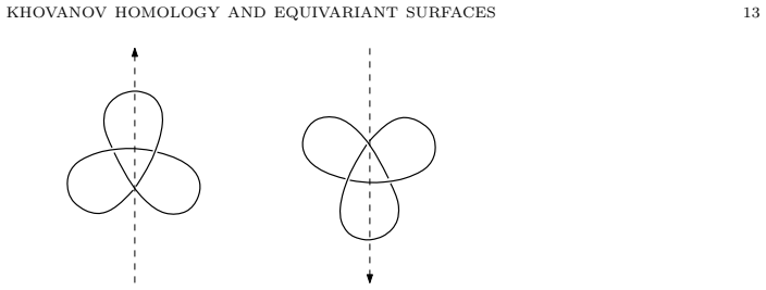
The load-bearing object is the reduced Borel complex $\widehat{\mathrm{Kcr}}^-_Q(K) = (\widehat{\mathrm{Kcr}}^-(K) \otimes \mathbb{F}[Q],\, \partial_Q = \partial + Q(1+\tau))$, built from Bar-Natan homology of a transvergent diagram, that is, a symmetric projection whose symmetry axis is visible. The extra variable $Q$ makes the involution part of the differential, so the invariant remembers the higher homotopy-commutation behavior of $\tau$ that ordinary $\tau$-complexes forget. Its localization at $u$ is $\mathbb{F}[u,u^{-1},Q]$, and the degrees in which $u$-nontorsion classes appear define the $\mathrm{es}_{Q,A,B}$ invariants. Invariance is proved by an explicit analysis of equivariant Reidemeister moves M1, M2, and M3; locality of connected equivariant cobordism maps is what produces the genus bounds.
What would settle it
Run the enumeration described in Lemma 6.13 on a transvergent diagram of $J=17\mathrm{nh}74$ and check for a grading-shift-zero local map from the five-generator complex $C_Q$ into $\widehat{\mathrm{Kcr}}^-_Q(J)$; absence of such a map would break Lemma 6.13 and the bound $\mathrm{eg}_4(\#^mJ)\ge\lceil m/2\rceil$.
Extended reading notes
Core claim
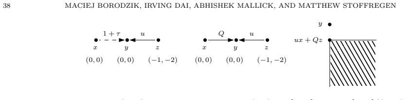
This paper's central discovery is that the Borel complex $\widehat{\mathrm{Kc}}^-_Q(L) = (\widehat{\mathrm{Kc}}^-(L) \otimes \mathbb{F}[Q],\, \partial_Q = \partial + Q(1+\tau))$ is a well-defined invariant of an involutive link up to Sakuma equivalence, and that an equivariant cobordism $\Sigma$ induces a local map on the reduced Borel complex $\widehat{\mathrm{Kcr}}^-_Q$ with grading shift $(0,-2g(\Sigma))$. The localization condition $u^{-1}H_*(\widehat{\mathrm{Kcr}}^-_Q(K)) \cong \mathbb{F}[u,u^{-1},Q]$ yields refined numerical invariants $\mathrm{es}_{Q,A,B}(K)$ satisfying the genus bound $\mathrm{es}_{Q,A,B}(K_1) - 2g(\Sigma) \le \mathrm{es}_{Q,A,B}(K_2)$. The main theorem is obtained by computing enough of the Borel complex of $J=17\mathrm{nh}74$: it contains a fixed five-generator subcomplex $C_Q$, and the $m$-fold connected sum of that subcomplex has $\mathrm{es}_{Q,m,m+1}(C_Q^{\otimes m}) \ge 2\lceil m/2\rceil$. The connected-sum formula is proved through Koszul duality, and a stabilization argument with the symmetric pair of slice disks for $J$ shows $\mathrm{eig}_4(\#^m J) \le 1$.
Load-bearing premise
The load-bearing premise is that every strongly invertible link and every equivariant cobordism can be equivariantly isotoped into the special symmetric diagram or movie form used here, with all the deferred genericity and move-level checks supplied rigorously; if any part of that fails, the Borel and mixed invariants are not known to be well-defined.
Editorial extensions
If this is right
- For the knot $J=17\mathrm{nh}74$, each connected sum $\#^m J$ satisfies $\mathrm{eg}_4(\#^m J)\ge\lceil m/2\rceil$ and $\mathrm{eig}_4(\#^m J)\le1$, so the two symmetric slice genera differ and the gap is unbounded.
- The invariants $\mathrm{es}_{Q,A,B}(K)$ are equivariant concordance invariants and obey $\mathrm{es}_{Q,A,B}(K_1)-2g(\Sigma)\le \mathrm{es}_{Q,A,B}(K_2)$ for equivariant cobordisms, strictly refining the earlier mapping-cone invariants.
- Because only genuine equivariant cobordisms induce Borel cobordism maps, the Borel invariants can distinguish the true equivariant slice genus from the isotopy-equivariant one; the mapping-cone style invariants cannot.
- The mixed complex, whose Q-equivalence class is invariant and which carries local equivariant cobordism maps, records the Lobb-Watson axis filtration and gives a route to equivariant genus bounds for knots whose $\tau$ action on homology is trivial.
- An equivariantly squeezed knot must have $\mathrm{es}(K)=s(K)$; in particular the strongly invertible knot $10_{141}$ is not equivariantly squeezed.
Reading between the lines
- Beyond the paper, the unbounded gap mechanism is portable: any knot whose reduced Borel complex contains a local image of the five-generator model $C_Q$ will produce the same growth under connected sums, so the phenomenon should occur in infinite families rather than in a single example.
- Beyond the paper, the Koszul-duality connected-sum formula suggests that equivariant Khovanov connected sums are governed by the full $\tau$-complexes of the factors, not their Borel complexes alone, which may create computational shortcuts for connected-sum computations.
- Beyond the paper, a direct testable extension is to compute the Q-equivalence classes of mixed complexes for small strongly invertible knots, especially ones whose $\tau$ action on Khovanov homology is trivial, to see whether the axis filtration alone distinguishes involutions that the Borel construction cannot yet distinguish.
Editorial analysis
A structured set of objections, weighed in public.
Referee Report
Summary. The paper develops a Bar-Natan homology refinement for involutive links. The main construction is the Borel complex Kc_Q(L) = (Kc^-(L) ⊗ F[Q], ∂ + Q(1+τ)), whose homotopy type is asserted to be invariant under Sakuma equivalence (Theorem 1.1), and which supports cobordism maps for equivariant cobordisms. From the reduced Borel complex the authors define numerical invariants es_Q and es_{Q,A,B} that bound the genus of equivariant cobordisms (Theorem 1.2). The principal application is Theorem 1.3: for the strongly invertible knot J = 17nh74, eg_4(#mJ) ≥ ⌈m/2⌉ while eig_4(#mJ) ≤ 1 for all m, exhibiting an arbitrarily large gap between the equivariant and isotopy-equivariant slice genus. The proof combines a local computation for J (Lemma 6.13), a connected-sum formula for Borel complexes obtained via Koszul duality (Theorem 6.25), a growth calculation for tensor powers (Lemma 6.30), and a topological stabilization argument (Lemma 6.32). The paper also develops mixed complexes to incorporate the Lobb–Watson filtration.
Significance. If the main theorems are correct, this is a substantial contribution: it gives the first proof that equivariant slice genus and isotopy-equivariant slice genus can differ, and that the gap can be arbitrarily large. The invariant is genuinely new in that it records higher homotopy-commutation data of the involution rather than only the homological action, and the paper explicitly identifies why Sano-style mapping-cone invariants, which are functorial for isotopy-equivariant cobordisms, cannot see this separation. The paper is also commendably concrete: it provides a computational program [BO25], detailed small examples, and falsifiable numerical predictions. The main theorems are stated carefully, and the algebraic framework for connected sums via Koszul duality is a useful and natural tool. The significance is, however, conditional on the postponed equivariant genericity statements and on the hand-verified enumeration in the key example.
major comments (3)
- [Section 2.2 (after Definition 2.9), Theorem 2.10, Definition 2.12] The well-definedness of the Borel complex and of the equivariant cobordism maps is load-bearing for Theorems 1.1, 1.2, and 1.3, but it depends on deferred genericity statements. The paper explicitly states that rigorous proofs of the existence of transvergent diagrams for involutive links, the completeness of the equivariant Reidemeister move set, including the I-move and R-move, and the existence of equivariantly generic cobordism movies will appear in [BDMS25]. Since Theorem 1.3 cannot hold if Kc_Q is not an invariant, these statements are not peripheral. A complete proof of these genericity results, or a published reference containing them, is required before the central claim can be regarded as established.
- [Section 5.3, M3 move] The invariance of Kc_Q under the M3 move is proved by a mapping-cone argument followed by a reduction to Bar-Natan's tangle category. The final step asserts that the constructed map F is, up to homotopy, the unique map coming from a morphism in Kob(R). This requires checking that the mapping-cone identifications are compatible with the tangle-category functor at each stage, not just that the tangles are simple. The paragraph currently gives only a heuristic justification; please spell out the naturality diagram that identifies the cone of the Borel complexes with the image under Kc^- of the corresponding cone in Kob(R). As written, the M3 invariance proof has a gap.
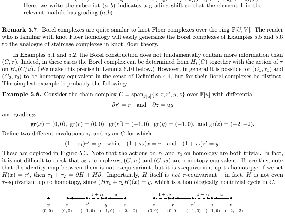
- [Section 6.3, Lemma 6.13 and Example 4.17] The lower bound in Theorem 1.3 depends on the existence of a local map from the complex C_Q of Example 5.9 into Kcr_Q(J). Lemma 6.13 rests on an 'exhaustive analysis' of the possible differential components X_i, Y_i, Z_i satisfying (6.14) and ∂_Q^2 = 0, but the enumeration is summarized rather than fully documented. Similarly, Example 4.17 refers to a 'straightforward but tedious exercise' enumerating extensions of τ. Because a single missed differential component could change the local equivalence class and hence the es_Q invariants, the argument is load-bearing. Please provide a complete case analysis or a machine-checkable verification for the enumeration.
minor comments (5)
- [Section 1.4] There is a typo: 'refinemenet' should be 'refinement.'
- [Section 6.5.3, Lemma 6.28] The statement of Lemma 6.28 contains a likely typo in the tensor-product direction: from the proof and from the use in Lemma 6.31, the conclusion should involve a local map Y1 ⊗ Y2 → Y1' ⊗ Y2' (with the appropriate ⊗_B product), not 'Y1 ⊗ Y1' → Y2 ⊗ Y2'.
- [Section 6.6, Lemma 6.30] In the displayed chain Σ_{i=0}^{⌊m/2⌋} u^{m-i} Q^{2i} x_i, the elements x_i are never defined. Presumably they denote suitable tensor-product generators in (C_Q)^{⊗m}; please define them explicitly, as this is the cycle used to prove the growth of es_Q.
- [Section 3.2] The notation 'dKcr_p(D)' and 'dKcr_un(D)' appears to be introduced without definition; it presumably means Kcr_p(D)/(u=0), but this should be stated.
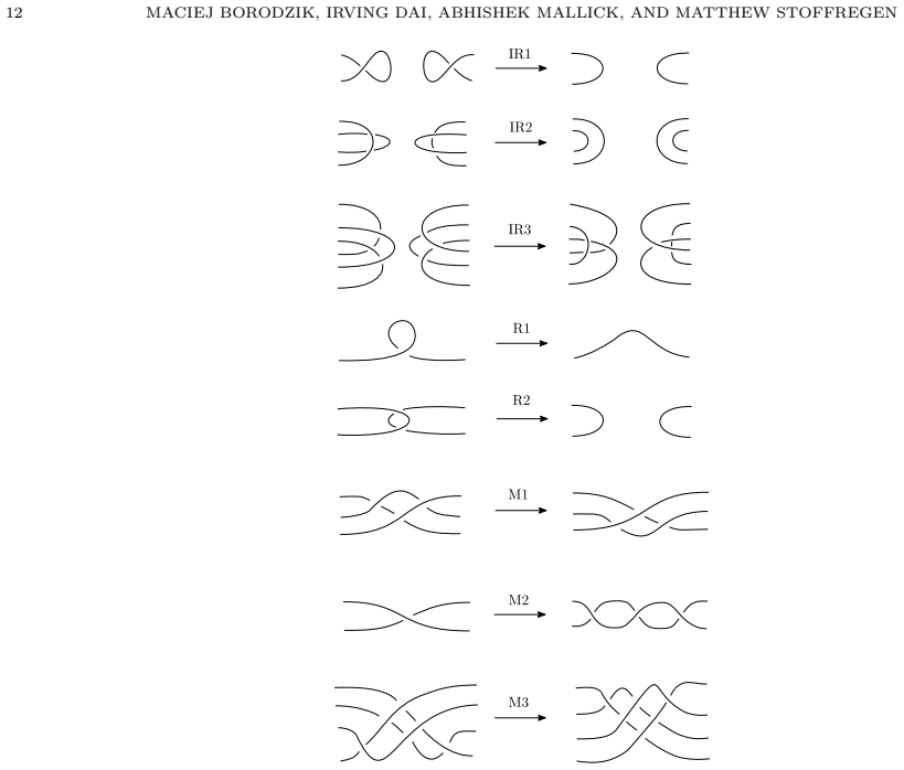
- [Section 2.2, Figure 2.2 and Theorem 2.10] Theorem 2.10 refers to moves '(IR-1) through (M-3)' in Figure 2.2, but the figure is not annotated with the move names here. Please label the moves explicitly so that the later references to M1, M2, and M3 in Section 5.3 can be checked.
Circularity Check
Deferred genericity results in [BDMS25] are load-bearing for the Borel invariant's well-definedness, but no fitted-input or definitional circularity appears in the algebraic core.
-
self citation load bearing
[Section 2.2, immediately after Definition 2.9]
"To the best of our knowledge, many genericity results regarding diagrams of strongly invertible links have been stated, but rigorous proofs have not appeared in the literature. A detailed, Morse-theoretical approach to diagrams of strongly invertible links will be given in our forthcoming paper [BDMS25]."
The invariance of the Borel complex Kc_Q (Theorem 1.1), and hence the esQ bound (Theorem 1.2) and the lower bound eg4(#mJ) >= ceil(m/2) (Lemma 6.31), presuppose that every involutive link can be represented by a transvergent diagram and every equivariant cobordism by an equivariant movie. These are not proved here; the paper explicitly defers them to the same authors' forthcoming [BDMS25]. The central theorem therefore rests on an unverified self-citation rather than a result established in this paper or by independent external work.
-
self citation load bearing
[Section 2.2, proof of Theorem 2.10]
"Except for the I-move, the claim is shown in [LW21, Theorem 2.3]. The I-move in the non-equivariant setting is discussed e.g. in [MWW22], where it leads to the sweep-around move. To the best of our knowledge, the I-move has not been studied in the equivariant setting. We refer to [BDMS25] for a detailed description."
Theorem 1.1 claims invariance of Kc_Q up to Sakuma equivalence. That equivalence is implemented by the move set of Theorem 2.10, whose I-move (the one move specific to passing through infinity, needed for the non-R3 part of Sakuma equivalence) is deferred to [BDMS25]. Since the same authors also defer the genericity results, the well-definedness of the Borel invariant is supported by an unproved self-citation chain; if the I-move statement fails, the lower genus bound in Theorem 1.3 loses its invariance.
full rationale
No fitted-input circularity, no definitional reduction, and no renaming of a known result occur in the algebraic argument. The esQ, esQ,A,B invariants are defined directly from the homology of the Borel complex; the genus bound follows from the monotonicity of these invariants under equivariant cobordism maps, and the connected-sum lower bound is computed from explicit complexes C^m_Q in Lemma 6.29, not from any parameter fitted to the data. The eig4(#mJ) <= 1 bound is a separate geometric stabilization argument using external results [CP21, CP23]. The only load-bearing weakness is the paper's explicit dependence on its own forthcoming [BDMS25] for the genericity of transvergent diagrams, the completeness of the equivariant move set (I-move), and equivariant movie decompositions. Those inputs are prerequisites for Kc_Q and esQ to be well-defined invariants, so if they fail the central claim collapses. Because these are unverified self-citations rather than independent theorems, the paper is not fully self-contained, though the identity of the failure is a geometric gap, not a circular definition. Score 4 reflects a load-bearing but non-definitional reliance on own unpublished work; the algebraic core, once the geometry is supplied, is not circular.
Assumptions & free parameters
assumptions (5)
- standard math Resolved Smith conjecture: the fixed-point set of any orientation-preserving involution on S3 with one-dimensional fixed set is an unknot, conjugate to the standard rotation.
- domain assumption Every involutive link up to Sakuma equivalence has a transvergent diagram, and every equivariant cobordism has an equivariantly generic movie presentation.
- standard math Bar-Natan homology is invariant under Reidemeister moves and functorial for cobordisms, including isotopy invariance of cobordism maps.
- domain assumption The I-move and the equivariant Reidemeister move classification for transvergent diagrams (Theorem 2.10) is correct, including the I-move case not previously studied.
- standard math Standard 4-manifold facts: pi1(B4 minus a slice disk) is Z, and homotopy of properly embedded arcs rel boundary implies isotopy.
Cite this review
Pith. "Pith review of Khovanov homology and equivariant surfaces." pith.science (2026). https://pith.science/paper/7XQS7XG5
@misc{pith2026250713642,
  author       = {Pith},
  title        = {Pith review of: Khovanov homology and equivariant surfaces},
  year         = {2026},
  howpublished = {\url{https://pith.science/paper/7XQS7XG5}},
  note         = {Machine review of arXiv:2507.13642}
}
read the original abstract
We introduce a refinement of Bar-Natan homology for involutive links, extending the work of Lobb-Watson and Sano. We construct a new suite of numerical invariants and derive bounds for the genus of equivariant cobordisms between strongly invertible knots. Our invariants show that the difference between the equivariant slice genus and isotopy-equivariant slice genus can be arbitrarily large, whereas previously these were not known to differ.
Figures


Figures from the paper (58 more)











Reference graph
Works this paper leans on
-
[1]
Antonio Alfieri and Keegan Boyle, Strongly invertible knots, invariant surfaces, and the A tiyah- S inger signature theorem , Michigan Math. J. 74 (2024), no. 4, 845--861. 4792563
work page 2024
-
[2]
Maciej Borodzik, Irving Dai, Abhishek Mallick, and Matthew Stoffregen, Strongly invertible links via M orse theory , 2025, in preparation
work page 2025
-
[3]
Maciej Borodzik and Stefan Friedl, On the algebraic unknotting number, Trans. London Math. Soc. 1 (2014), no. 1, 57--84. 3296484
work page 2014
-
[4]
Alexander Beilinson, Victor Ginzburg, and Wolfgang Soergel, Koszul duality patterns in representation theory, J. Amer. Math. Soc. 9 (1996), no. 2, 473--527. 1322847
1996
-
[5]
Keegan Boyle and Ahmad Issa, Equivariant 4-genera of strongly invertible and periodic knots, J. Topol. 15 (2022), no. 3, 1635--1674. 4461855
work page 2022
-
[6]
Knot Theory Ramifications 19 (2010), no
Christian Blanchet, An oriented model for K hovanov homology , J. Knot Theory Ramifications 19 (2010), no. 2, 291--312. 2647055
2010
-
[7]
Bloom, Odd K hovanov homology is mutation invariant , Math
Jonathan M. Bloom, Odd K hovanov homology is mutation invariant , Math. Res. Lett. 17 (2010), no. 1, 1--10. 2592723
work page 2010
-
[8]
John A Baldwin, Adam Simon Levine, and Sucharit Sarkar, Khovanov homology and knot floer homology for pointed links, Journal of Knot Theory and Its Ramifications 26 (2017), no. 02, 1740004
work page 2017
Show all 57 references
-
[9]
Dror Bar-Natan, Khovanov's homology for tangles and cobordisms, Geom. Topol. 9 (2005), 1443--1499. 2174270
2005
-
[10]
Maciej Borodzik and Jacek Olesiak, Khocomp, Available at https://github.com/mcboro/Khocomp, 2025, C++ program to compute equivariant Khovanov homology
2025
-
[11]
3, 1233--1309
Maciej Borodzik, Wojciech Politarczyk, and Marithania Silvero, Khovanov homotopy type, periodic links and localizations, Mathematische Annalen 380 (2021), no. 3, 1233--1309
2021
-
[12]
339--414
Maciej Borodzik, Wojciech Politarczyk, and Ramazan Yozgyur, Khovanov- R ozansky sl _n -homology for periodic links , 2025, pp. 339--414
2025
-
[13]
Bredon, Introduction to compact transformation groups, Pure and Applied Mathematics, Vol
Glen E. Bredon, Introduction to compact transformation groups, Pure and Applied Mathematics, Vol. 46, Academic Press, New York-London, 1972. 0413144
1972
-
[14]
Jae Choon Cha and Ki Hyoung Ko, On equivariant slice knots, Proc. Amer. Math. Soc. 127 (1999), no. 7, 2175--2182. 1605928
1999
-
[15]
Anthony Conway and Mark Powell, Characterisation of homotopy ribbon discs, Adv. Math. 391 (2021), Paper No. 107960, 29. 4300918
2021
-
[16]
, Embedded surfaces with infinite cyclic knot group, Geom. Topol. 27 (2023), no. 2, 739--821. 4589564
2023
-
[17]
Marius Crainic, On the perturbation lemma, and deformations, arXiv preprint math/0403266 (2004)
2004 arXiv
-
[18]
Daren Chen and Hongjian Yang, The flip map and involutions on khovanov homology, 2025, preprint, arxiv:2506.00824
2025
-
[19]
Irving Dai, Matthew Hedden, and Abhishek Mallick, Corks, involutions, and H eegaard F loer homology , J. Eur. Math. Soc. (JEMS) 25 (2023), no. 6, 2319--2389. 4592871
2023
-
[20]
Nathan M Dunfield, Robert Lipshitz, and Dirk Schuetz, Local equivalence and refinements of R asmussen's s-invariant , arXiv preprint arXiv:2312.09114 (2023)
2023
-
[21]
Irving Dai, Abhishek Mallick, and Matthew Stoffregen, Equivariant knots and knot F loer homology , J. Topol. 16 (2023), no. 3, 1167--1236. 4638003
2023
-
[22]
Davis and Swatee Naik, Alexander polynomials of equivariant slice and ribbon knots in S^3 , Trans
James F. Davis and Swatee Naik, Alexander polynomials of equivariant slice and ribbon knots in S^3 , Trans. Amer. Math. Soc. 358 (2006), no. 7, 2949--2964. 2216254
2006
-
[23]
Peter Feller, Lukas Lewark, and Andrew Lobb, Squeezed knots, 2022, preprint, arXiv:2202.12289
2022
-
[24]
Freedman and Frank Quinn, Topology of 4-manifolds, Princeton Mathematical Series, vol
Michael H. Freedman and Frank Quinn, Topology of 4-manifolds, Princeton Mathematical Series, vol. 39, Princeton University Press, Princeton, NJ, 1990. 1201584
1990
-
[25]
Kyle Hayden, C orks, covers, and complex curves , 2021, preprint, arXiv:2107.06856
2021 arXiv
-
[26]
Kristen Hendricks and Ciprian Manolescu, Involutive H eegaard F loer homology , Duke Math. J. 166 (2017), no. 7, 1211--1299
2017
-
[27]
(N.S.) 24 (2018), no
Kristen Hendricks, Ciprian Manolescu, and Ian Zemke, A connected sum formula for involutive H eegaard F loer homology , Selecta Math. (N.S.) 24 (2018), no. 2, 1183--1245
2018
-
[28]
Reine Angew
Kyle Hayden and Isaac Sundberg, Khovanov homology and exotic surfaces in the 4-ball, J. Reine Angew. Math. 809 (2024), 217--246. 4726569
2024
-
[29]
Magnus Jacobsson, An invariant of link cobordisms from K hovanov homology , Algebr. Geom. Topol. 4 (2004), 1211--1251. 2113903
2004
-
[30]
Mikhail Khovanov, A categorification of the J ones polynomial , Duke Math. J. 101 (2000), no. 3, 359--426. 1740682
2000
-
[31]
Sadayoshi Kojima and Masayuki Yamasaki, Some new invariants of links, Invent. Math. 54 (1979), no. 3, 213--228. 553219
1979
-
[32]
2, 554--586
Eun Soo Lee, An endomorphism of the K hovanov invariant , Advances in Mathematics 197 (2005), no. 2, 554--586
2005
-
[33]
Adam Simon Levine, Tye Lidman, and Lisa Piccirillo, New constructions and invariants of closed exotic 4-manifolds, arXiv preprint arXiv:2307.08130 (2023)
2023 arXiv
-
[34]
Robert Lipshitz and Sucharit Sarkar, A refinement of R asmussen's s -invariant , Duke Math. J. 163 (2014), no. 5, 923--952. 3189434
2014
-
[35]
12, 8807--8849
, A mixed invariant of nonorientable surfaces in equivariant K hovanov homology , Transactions of the American Mathematical Society 375 (2022), no. 12, 8807--8849
2022
-
[36]
, Khovanov homology of strongly invertible knots and their quotients, Frontiers in geometry and topology, Proc. Sympos. Pure Math., vol. 109, Amer. Math. Soc., Providence, RI, [2024] 2024, pp. 157--182. 4772951
2024
-
[37]
Andrew Lobb and Liam Watson, A refinement of K hovanov homology , Geom. Topol. 25 (2021), no. 4, 1861--1917. 4286365
2021
-
[38]
Morgan and Hyman Bass, The S mith conjecture , Pure Appl
John W. Morgan and Hyman Bass, The S mith conjecture , Pure Appl. Math., vol. 112, Academic Press, Orlando, FL, 1984, pp. 3--6. 758460
1984
-
[39]
Alice Merz, The A lexander and M arkov theorems for strongly involutive links , 2024, preprint, arXiv: 2406.13592
2024 arXiv
-
[40]
Ciprian Manolescu and Peter Ozsv\'ath, Heegaard F loer homology and integer surgeries on links , 2010, preprint, arXiv:1011.1317v3
2010
-
[41]
Miller and Mark Powell, Strongly invertible knots, equivariant slice genera, and an equivariant algebraic concordance group, J
Allison N. Miller and Mark Powell, Strongly invertible knots, equivariant slice genera, and an equivariant algebraic concordance group, J. Lond. Math. Soc. (2) 107 (2023), no. 6, 2025--2053. 4598178
2023
-
[42]
Kunio Murasugi, On periodic knots, Comment. Math. Helv. 46 (1971), 162--174. 292060
1971
-
[43]
Scott Morrison, Kevin Walker, and Paul Wedrich, Invariants of 4-manifolds from K hovanov- R ozansky link homology , Geom. Topol. 26 (2022), no. 8, 3367--3420. 4562565
2022
-
[44]
Swatee Naik, Periodicity, genera and A lexander polynomials of knots , Pacific J. Math. 166 (1994), no. 2, 357--371. 1313460
1994
-
[45]
Ozsv\'ath, Jacob Rasmussen, and Zolt\'an Szab\'o, Odd K hovanov homology , Algebr
Peter S. Ozsv\'ath, Jacob Rasmussen, and Zolt\'an Szab\'o, Odd K hovanov homology , Algebr. Geom. Topol. 13 (2013), no. 3, 1465--1488. 3071132
2013
-
[46]
2, 419--447
Jacob Rasmussen, Khovanov homology and the slice genus, Inventiones Mathematicae 182 (2010), no. 2, 419--447
2010
-
[47]
176--196
Makoto Sakuma, On strongly invertible knots, Algebraic and topological theories ( K inosaki, 1984), Kinokuniya, Tokyo, 1986, pp. 176--196. 1102258
1984
-
[48]
Taketo Sano, Involutive K hovanov homology and equivariant knots , 2025, preprint, arxiv:2404.08568
2025
-
[49]
Dirk Sch\"utz, On an integral version of the R asmussen invariant , Michigan Math. J. 75 (2025), no. 1, 65--88. 4873797
2025
-
[50]
Isaac Sundberg and Jonah Swann, Relative K hovanov- J acobsson classes , Algebr. Geom. Topol. 22 (2022), no. 8, 3983--4008. 4562563
2022
-
[51]
Matthew Stoffregen and Melissa Zhang, Localization in K hovanov homology , Geom. Topol. 28 (2024), no. 4, 1501--1585. 4777698
2024
-
[52]
Knot Theory Ramifications 29 (2020), no
Pierre Vogel, Functoriality of K hovanov homology , J. Knot Theory Ramifications 29 (2020), no. 4, 2050020, 66. 4096813
2020
-
[53]
U ber I nvolutionen der 3 - S ph\
Friedhelm Waldhausen, \" U ber I nvolutionen der 3 - S ph\" a re , Topology 8 (1969), 81--91. 236916
1969
-
[54]
Liam Watson, Khovanov homology and the symmetry group of a knot, Adv. Math. 313 (2017), 915--946. 3649241
2017
-
[55]
Wehrli, Mutation invariance of K hovanov homology over F_2 , Quantum Topol
Stephan M. Wehrli, Mutation invariance of K hovanov homology over F_2 , Quantum Topol. 1 (2010), no. 2, 111--128. 2657645
2010
-
[56]
Weibel, An introduction to homological algebra, Cambridge Studies in Advanced Mathematics, vol
Charles A. Weibel, An introduction to homological algebra, Cambridge Studies in Advanced Mathematics, vol. 38, Cambridge University Press, Cambridge, 1994. 1269324
1994
-
[57]
04, 1650014
Yuval Wigderson, The B ar- N atan theory splits , Journal of Knot Theory and Its Ramifications 25 (2016), no. 04, 1650014
2016
Reviewed August 6, 2026 · model on record in the stance chip above.
Discussion (0). Continue with ORCID to comment.