REVIEW 3 major objections 6 minor 43 references
Modeling microstructure price dynamics with symmetric Hawkes and diffusion model using ultra-high-frequency stock data
T0 review · 3 major / 6 minor · reviewed 2026-08-14 · deepseek-v4-flash
Pith's one-line read The symmetric Hawkes model, estimated from every tick-level mid-price move, gives volatility within about 15–25 percent of realized measures and a diffusion analogue with close distributional properties.
desk verdict Diffusion analogue is a useful idea with honest caveats, but the claimed closeness to Hawkes is not quantitatively established; deserves a serious referee and a revision. read the letter →
The pith
A machine-rendered reading of the paper's core claim, the machinery that carries it, and where it could break.
The reading
What carries the argument
The load-bearing object is the symmetric Hawkes process: a bivariate point process $(N_1,N_2)$ with exponential-decay intensities sharing baseline $\mu$, decay $\beta$, self-excitation $\alpha_s$, and mutual excitation $\alpha_c$, whose difference scaled by the tick size $\delta$ is the mid-price. Its tractability comes from two facts: fixing $\beta$ makes the log-likelihood concave in $(\mu,\alpha_s,\alpha_c)$, so the maximum can be located reliably; and the stationarity assumption $\lambda_1(0)=\lambda_2(0)=\mu\beta/(\beta-\alpha_s-\alpha_c)$ reduces the return variance to a closed formula. The diffusion analogue $dS_t=n_tdt+\sqrt{V_t}dW^s_t$, $dn_t=-\kappa_1 n_tdt+\phi\sqrt{V_t}dW^s_t$, $dV_t=\kappa_2(\theta-V_t)dt+\gamma\sqrt{V_t}dW^v_t$ with the parameter identities above carries the second half of the paper: it imports Heston-type square-root variance machinery, a leverage parameter $\rho$, and simulated maximum likelihood estimation into the tick-level setting.
What would settle it
Take a low-activity stock or day, simulate the fitted symmetric Hawkes process, and compare one-minute mid-price return densities with the diffusion analogue's Kolmogorov-forward density; a significant distributional distance would show the normal approximation fails at that time scale.
Extended reading notes
Core claim
On the paper's own terms, the central discovery is that the price process $S_t = S_0 + \delta(N_1(t)-N_2(t))$, with $N_1,N_2$ counting up and down moves of the mid-price and each intensity following a Hawkes process with common baseline $\mu$, decay $\beta$, self-excitation $\alpha_s$, and mutual excitation $\alpha_c$, can be estimated by maximum likelihood from ultra-high-frequency data. Under the stationarity condition $\lambda_1(0)=\lambda_2(0)=\mu\beta/(\beta-\alpha_s-\alpha_c)$, the return variance has the closed form $$\operatorname{Var}\left(\frac{S_t-S_0}{S_0}\right)=\frac{2\$delta^{2}$\lambda_1(0)}{$S_0^{2}$\$xi_1^{2}$}\left\{\$beta^{2}$t-\frac{2(\alpha_s-\alpha_c)\$\beta$}{\xi_1}($e^{{\xi_1 t}}$-1)+\frac{(\alpha_s-\alpha_c)^2}{2\xi_1}($e^{{2\xi_1 t}}$-1)\right\},$$ with $\xi_1=-\beta-\alpha_c+\alpha_s$, and this Hawkes volatility tracks TSRV and RRV on ten S&P 500 stocks with mean percentage errors typically in the 15–25 percent range. The companion claim is that replacing Poisson increments by Brownian increments over one-minute intervals produces the diffusion system $dS_t=n_tdt+\sqrt{V_t}dW^s_t$, $dn_t=-\kappa_1 n_tdt+\phi\sqrt{V_t}dW^s_t$, $dV_t=\kappa_2(\theta-V_t)dt+\gamma\sqrt{V_t}dW^v_t$, with $\kappa_1=b-a_s+a_c$, $\kappa_2=b-a_s-a_c$, $\theta=2bm\delta^2/(b-a_s-a_c)$, $\gamma=\delta(a_s+a_c)$, $\phi=a_s-a_c$, and $d[W^s,W^v]_t=\rho dt$; the paper reports that this diffusion has a very close distributional property to the Hawkes model, giving simpler variance and skewness formulas and a leverage parameter $\rho$.
Load-bearing premise
The load-bearing premise is that over a one-minute interval enough mid-price changes occur for the Poisson increments in the Hawkes process to be well approximated by normal (Brownian) increments; the paper gives no error bound for this replacement, and the diffusion model's very close distributional claim depends on it.
Editorial extensions
If this is right
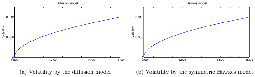
- Volatility can be estimated from as little as ten minutes of mid-price tick data, so the model produces an intraday volatility curve updated every ten minutes.
- The closed-form Hawkes variance formula lets practitioners reparametrize the likelihood directly in terms of annualized volatility and estimate it without first removing microstructure noise.
- If the diffusion analogue is accepted, variance, skewness, and leverage formulas follow from Itô calculus, making the tick-level model compatible with standard continuous-time tools.
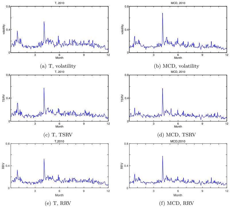
- The empirical comparison shows that the Hawkes volatility tracks TSRV and RRV daily, with mean percentage errors between the two measures staying around 15–25 percent for ten S&P 500 stocks.
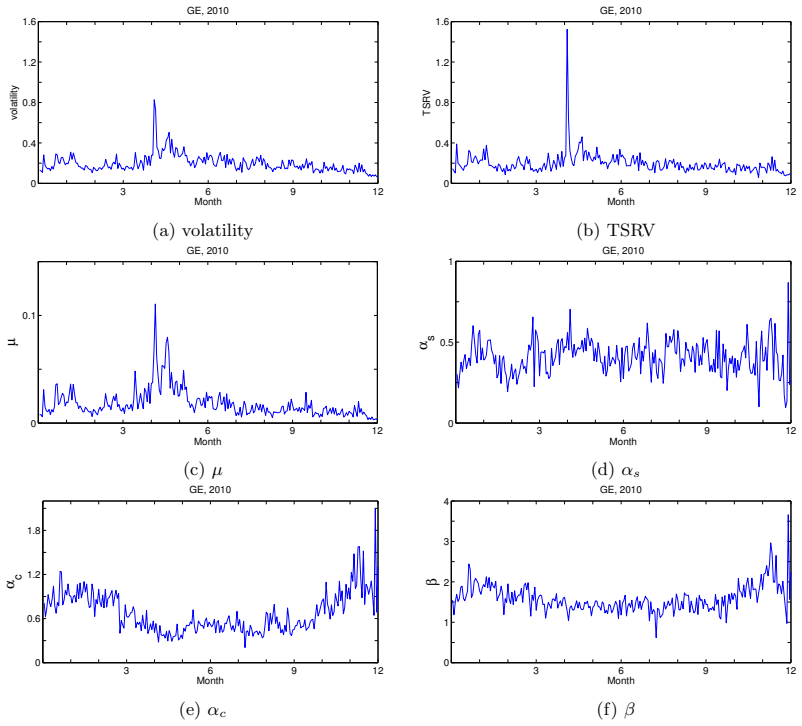
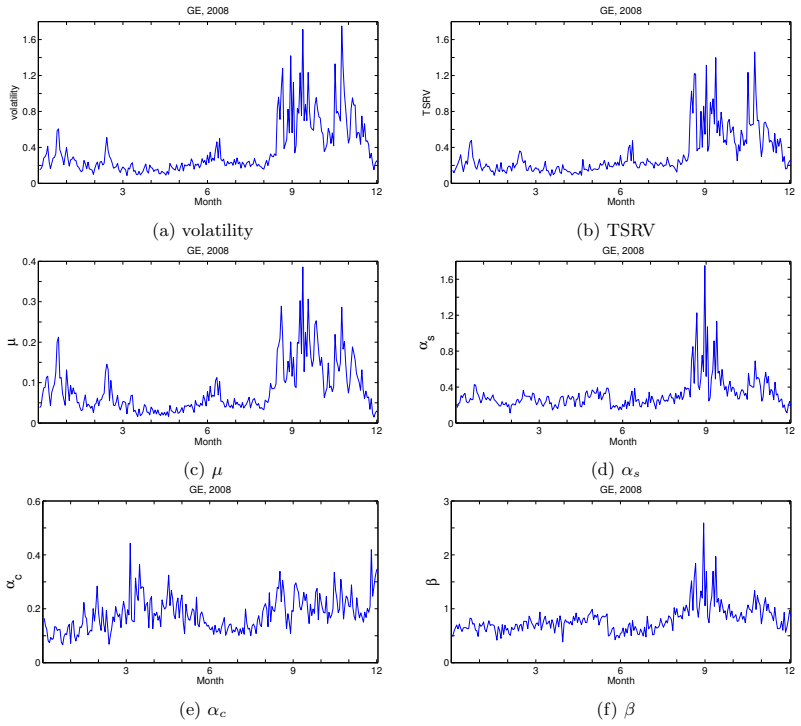
- The fully characterized Hawkes estimates show the symmetry assumptions are often reasonable, while cases like XOM in 2008 indicate persistence differences between self- and mutual excitation that a symmetric model cannot capture.
Reading between the lines
- A natural extension is to estimate the diffusion model on one-minute bins for less liquid names, where the normal approximation is most doubtful; if distributional closeness breaks down there, that would identify the shortest safe sampling scale.
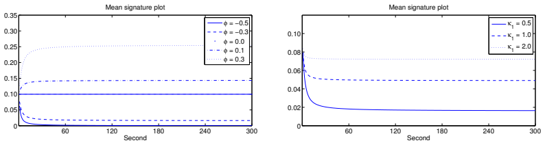
- The mean signature plot analysis implies that the sign of the parameter $\phi=a_s-a_c$ controls how realized variance responds to sampling frequency, and this directional prediction is directly checkable on the same high-frequency data.
- If the diffusion analogy holds, Heston-style option pricing formulas could be applied with parameters estimated from tick arrivals, connecting ultra-high-frequency estimation to derivatives pricing.
- The paper's 15–25 percent gap between Hawkes volatility and TSRV is left unexplained; allowing the baseline intensity to vary intraday in the likelihood would test whether parameter drift accounts for the gap.
Signed reviews
Editorial analysis
A structured set of objections, weighed in public.
Referee Report
Summary. The paper studies a symmetric bivariate Hawkes process for tick-level mid-price dynamics, estimates its parameters by maximum likelihood from ultra-high-frequency NYSE data for ten S&P 500 stocks, and compares the resulting Hawkes-based volatility with two-scale realized volatility (TSRV) and the Robert-Rosenbaum volatility (RRV). The empirical part reports daily and intraday parameter dynamics and finds that Hawkes volatility is generally within 15–25% of TSRV. The paper then proposes a continuous-time diffusion analogue of the Hawkes model, with state variables for price, drift, and variance, and derives closed-form variance and third-moment formulas. Parameter estimates for the diffusion model are obtained by simulated maximum likelihood. The central claim is that the diffusion analogue has 'very close distributional property' to the Hawkes model while offering analytical simplicity.
Significance. If the claims were fully established, the Hawkes-based volatility estimator would be a useful tool for intraday risk measurement using all tick arrivals, and the diffusion analogue would provide a tractable continuous-time model for high-frequency volatility and skewness. The paper has concrete strengths: the Hawkes likelihood estimation is standard and is checked in a simulation study; the variance derivations in the appendices are detailed and checkable; the empirical comparison with TSRV and RRV is extensive and includes an interesting intraday volatility application. The main weakness is that the diffusion analogue—a major advertised contribution—is supported only by a heuristic normal approximation with no error control, and the empirical diffusion estimates do not match the Hawkes volatilities well. The paper is therefore promising but requires substantial additional work before the central diffusion-analogy claim can be accepted.
major comments (3)
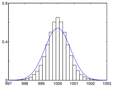
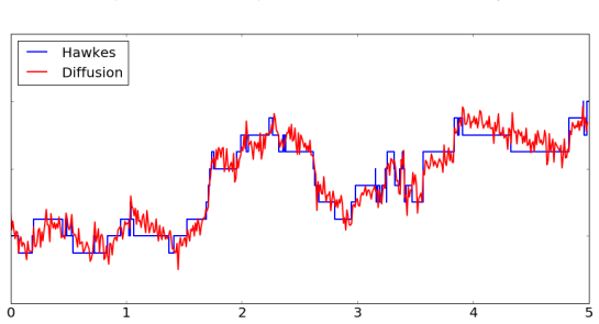
- [Section 3.1 and Section 3.3] The normal approximation underlying the diffusion analogue is not justified for the data actually used. Section 3.1 replaces Poisson increments by normal increments on the grounds that 'a sufficient number of price changes were observed during, e.g., one minute.' The paper's own estimates contradict this: for GE on 2011-01-03, Table 4 gives mu=0.0067, alpha_s=0.4661, alpha_c=1.3576, beta=2.2596, so the stationary intensity per direction is about 0.0347 per second, or about 4 mid-price changes per minute total; Table 5 gives roughly 5.6 per minute for T. A Poisson sum with mean 4–13 is not close to Gaussian, and no quantitative error bound is provided. Section 3.3 concedes the derivation is 'not a rigorous mathematical transform' and only 'to provide an intuition,' yet Section 3.4 uses the diffusion model as the working model for estimation. The 'very close distributional property' claim is therefore not supported for the low-intensity stocks in the empirical study; Figure 2 uses a high-intensity parameter setting (mu=0.09, 30-second horizon) and reports no error metric. Please provide a quantitative justification (e.g., a Berry-Esseen bound or a limit theorem with stationarity conditions) or explicitly restrict the claim to regimes where the normal approximation is verified.
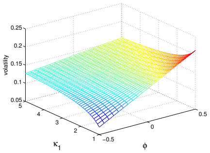
- [Section 3.1, parameter mapping after Eq. (9)] Part of the agreement between the diffusion model and the Hawkes model is by construction. The parameter relation theta = 2bm*delta^2/(b-as-ac) is chosen so that the long-run variance of the diffusion model, b^2 theta t/(S0^2 kappa1^2), exactly equals the long-run variance of the Hawkes model in Remark 2 when m=mu, as=alpha_s, ac=alpha_c, b=beta. Thus the asymptotic variance comparison after Proposition 4 is not independent evidence of distributional closeness; it is baked into the parameter mapping. The finite-time variance in Proposition 4 is a genuine derivation, but its agreement with Proposition 3 is shown in only one figure (Figure 3) and one parameter set. Please clarify in the text that the long-run variance match is by construction and present finite-time comparisons over a range of empirically calibrated parameters.
- [Section 4.5, Tables 8 and 4] The claimed empirical similarity between the diffusion-model estimates and the Hawkes estimates is not supported by the reported numbers. For GE in January 2011, Table 8 gives diffusion volatilities that are frequently much larger than the Hawkes H.vol in Table 4: on 0105 the diffusion volatility is 0.3661 versus 0.1339 for Hawkes, on 0104 it is 0.1546 versus 0.1139, and on 0110 it is 0.1739 versus 0.1520. Several diffusion estimates also have parameter values very different from the Hawkes estimates (e.g., ac=2.9568 on 0104 vs. alpha_c=1.3941 in Table 4). The text states that the results are 'similar' to the Hawkes model without providing a quantitative comparison, confidence intervals, or an explanation of the systematic discrepancy. Please either provide a proper comparison (e.g., ratio statistics, error bars, or a scatter plot) or temper the claim about the empirical similarity of the two models.
minor comments (6)
- [Abstract] The sentence 'This study examine the theoretical and empirical perspectives' should read 'This study examines'; the same grammatical issue appears in the introduction.
- [Section 2.3] There is a typo 'Haweks' in the paragraph introducing the symmetric model; it should be 'Hawkes'.
- [Section 2.4] The reported estimates for 'simulation set 1' in the text appear to actually be from simulation set 2 (alpha_s=0.6590 is close to the true alpha_s=0.65 of set 2, not the true alpha_s=0.4 of set 1). Also, 'alpha_c = 0.0.4864' contains a typo and should be '0.4864'.
- [Figure 2 and Section 3.2] The caption of Figure 2 says 'histogram of the Hawkes model price by the simulation with 30 seconds (right)' but the panel labels are not visible; please clarify which panel shows the density and which shows the histogram, and add a legend or labels.
- [Section 4.5] Tables 8 and 9 report diffusion parameter estimates without standard errors or any measure of simulation variability; because the simulated likelihood depends on random numbers, at least the seed or a small Monte Carlo standard error should be reported.
- [Appendix C] The likelihood form in Eq. (C.1) should define the log-likelihood function with the parameter vector explicitly; the notation L(θ,T) appears only later, and the text introduces 'the conditional cumulative distributions' with an unnumbered equation that is not referenced.
Circularity Check
No significant circularity: Hawkes volatility is derived from the model and benchmarked externally, while the diffusion model is a transparent analogy rather than a circular derivation.
full rationale
The paper's central volatility claim is not circular. Proposition 3 is derived in Appendix D from the symmetric Hawkes intensity dynamics and the stationarity condition, and it is cross-checked against Da Fonseca and Zaatour (2014a) with a noted difference in the exponential term. The empirical H.vol is a maximum-likelihood model output, not a fit to TSRV or RRV, which are independent realized-volatility benchmarks; the reported 15–25% differences are therefore informative. The diffusion section is explicitly an analogy: Section 3.1 constructs the parameter mapping (κ1, κ2, θ, γ, φ) so that the diffusion has the same eigenvalues and stationary variance as the Hawkes model, and Section 3.3 states the derivation is 'not a rigorous mathematical transform' and is meant only 'to provide an intuition not a mathematical proof.' The long-run variance agreement between Proposition 4 and Remark 2 is a transparent consequence of the θ calibration, not a hidden reuse of the target result, and the full variance formulas are not algebraically identical. Self-citations (Choe and Lee 2014a,b; Lee 2016) are used for defining third-moment variation and a moment-estimation method; Proposition 5 is proved in the appendix, so the central derivation does not rest on an unverified self-citation. The unquantified normal approximation for low-intensity stocks (e.g., GE with roughly 4–6 mid-price changes per minute) is a correctness and robustness limitation, not circularity.
Assumptions & free parameters
free parameters (6)
- mu (baseline intensity) =
e.g., 0.0067 to 0.0316 for GE January 2011 (Table 4)
- alpha_s (self-excitation coefficient) =
e.g., 0.42 to 0.70 for GE January 2011
- alpha_c (cross-excitation coefficient) =
e.g., 0.35 to 1.39 for GE January 2011
- beta (decay rate) =
e.g., 1.42 to 2.53 for GE January 2011
- Diffusion parameters m, as, ac, b, rho =
GE January 2011 values in Tables 8 and 9
- Hand-chosen model parameters for comparisons =
Figure 2: m=0.09, as=0.6, ac=0.3, b=2.5, delta=0.2; Figure 3: as=1.2, ac=0.3, b=2.2, m=0.01, delta/S0=0.002
assumptions (6)
- standard math Spectral radius of the branching matrix Q is less than 1 (qs+qc<1) for the Hawkes process to be well defined.
- domain assumption The intensity processes are in stationarity at time 0: lambda1(0)=lambda2(0)=mu*beta/(beta-alpha_s-alpha_c), and later V0=theta, n0=0.
- ad hoc to paper Poisson increments are approximated by normal increments at the one-minute scale.
- ad hoc to paper The diffusion model SDE is postulated as an analogy rather than derived as a limit.
- domain assumption Data preprocessing: price changes are multiples of half the minimal spread, larger changes are decomposed into successive minimal moves, and 1-second timestamps are redistributed uniformly.
- domain assumption The variance process remains nonnegative and the correlation rho is treated as constant.
invented entities (1)
-
Diffusion analogue process (S_t, n_t, V_t)
Cite this review
Pith. "Pith review of Modeling microstructure price dynamics with symmetric Hawkes and diffusion model using ultra-high-frequency stock data." pith.science (2026). https://pith.science/paper/7Y4KRDUY
@misc{pith2026190805089,
  author       = {Pith},
  title        = {Pith review of: Modeling microstructure price dynamics with symmetric Hawkes and diffusion model using ultra-high-frequency stock data},
  year         = {2026},
  howpublished = {\url{https://pith.science/paper/7Y4KRDUY}},
  note         = {Machine review of arXiv:1908.05089}
}
read the original abstract
This study examine the theoretical and empirical perspectives of the symmetric Hawkes model of the price tick structure. Combined with the maximum likelihood estimation, the model provides a proper method of volatility estimation specialized in ultra-high-frequency analysis. Empirical studies based on the model using the ultra-high-frequency data of stocks in the S\&P 500 are performed. The performance of the volatility measure, intraday estimation, and the dynamics of the parameters are discussed. A new approach of diffusion analogy to the symmetric Hawkes model is proposed with the distributional properties very close to the Hawkes model. As a diffusion process, the model provides more analytical simplicity when computing the variance formula, incorporating skewness and examining the probabilistic property. An estimation of the diffusion model is performed using the simulated maximum likelihood method and shows similar patterns to the Hawkes model.
Figures

Figures from the paper (10 more)




Reference graph
Works this paper leans on
-
[1]
A \" t-Sahalia, Y., Cacho-Diaz, J., and Laeven, R. J. (2010). Modeling financial contagion using mutually exciting jump processes. Technical report, National Bureau of Economic Research
work page 2010
-
[2]
A \" t-Sahalia, Y. et al. (2008). Closed-form likelihood expansions for multivariate diffusions. The Annals of Statistics , 36(2):906--937
work page 2008
-
[3]
Ait-Sahalia, Y., Fan, J., and Li, Y. (2013). The leverage effect puzzle: Disentangling sources of bias at high frequency. Journal of Financial Economics , 109:224--249
work page 2013
-
[4]
A \" t-Sahalia, Y., Mykland, P. A., and Zhang, L. (2005). How often to sample a continuous-time process in the presence of market microstructure noise. Review of Financial studies , 18:351--416
work page 2005
-
[5]
A \" t-Sahalia, Y., Mykland, P. A., and Zhang, L. (2011). Ultra high frequency volatility estimation with dependent microstructure noise. Journal of Econometrics , 160:160--175
work page 2011
-
[6]
G., Bollerslev, T., Diebold, F
Andersen, T. G., Bollerslev, T., Diebold, F. X., and Labys, P. (2003). Modeling and forecasting realized volatility. Econometrica , 71:579--625
work page 2003
-
[7]
Bacry, E., Dayri, K., and Muzy, J.-F. (2012). Non-parametric kernel estimation for symmetric Hawkes processes. application to high frequency financial data. The European Physical Journal B-Condensed Matter and Complex Systems , 85:1--12
work page 2012
-
[8]
Bacry, E., Delattre, S., Hoffmann, M., and Muzy, J.-F. (2013). Modelling microstructure noise with mutually exciting point processes. Quantitative Finance , 13:65--77
work page 2013
Show all 43 references
-
[9]
and Muzy, J.-F
Bacry, E. and Muzy, J.-F. (2014). Hawkes model for price and trades high-frequency dynamics. Quantitative Finance , 14:1147--1166
2014
-
[10]
Barndorff-Nielsen, O. E. and Shephard, N. (2002a). Econometric analysis of realized volatility and its use in estimating stochastic volatility models. Journal of the Royal Statistical Society: Series B (Statistical Methodology) , 64:253--280
2002
-
[11]
Barndorff-Nielsen, O. E. and Shephard, N. (2002b). Estimating quadratic variation using realized variance. Journal of Applied Econometrics , 17:457--477
2002
-
[12]
and Hautsch, N
Bauwens, L. and Hautsch, N. (2009). Modelling financial high frequency data using point processes. In Handbook of Financial Time Series , pages 953--979. Springer Berlin Heidelberg
2009
-
[13]
Bollerslev, T., Gibson, M., and Zhou, H. (2011). Dynamic estimation of volatility risk premia and investor risk aversion from option-implied and realized volatilities. Journal of econometrics , 160(1):235--245
2011
-
[14]
Bowsher, C. G. (2007). Modelling security market events in continuous time: Intensity based, multivariate point process models. Journal of Econometrics , 141:876--912
2007
-
[15]
Brandt, M. W. and Santa-Clara, P. (2002). Simulated likelihood estimation of diffusions with an application to exchange rate dynamics in incomplete markets. Journal of financial economics , 63:161--210
2002
-
[16]
Br \'e maud, P. (1981). Point Processes and Queues : Martingale Dynamics . Springer
1981
-
[17]
Broyden, C. G. (1970). The convergence of a class of double-rank minimization algorithms 1. general considerations. IMA Journal of Applied Mathematics , 6:76--90
1970
-
[18]
Choe, G. H. and Lee, K. (2014a). Conditional correlation in asset return and garch intensity model. AStA Advances in Statistical Analysis , 98:197--224
2014
-
[19]
Choe, G. H. and Lee, K. (2014b). High moment variations and their application. Journal of Futures Markets , 34:1040--1061
2014
-
[20]
and Zaatour, R
Da Fonseca, J. and Zaatour, R. (2014a). Clustering and mean reversion in a Hawkes microstructure model. Journal of Futures Markets , 35:813--838
2014
-
[21]
and Zaatour, R
Da Fonseca, J. and Zaatour, R. (2014b). Hawkes process: Fast calibration, application to trade clustering, and diffusive limit. Journal of Futures Markets , 34:548--579
2014
-
[22]
Daley, D. J. and Vere-Jones, D. (2003). An introduction to the theory of point processes , volume 1. Springer
2003
-
[23]
and Zhao, H
Dassios, A. and Zhao, H. (2012). Ruin by dynamic contagion claims. Insurance: Mathematics and Economics , 51:93--106
2012
-
[24]
El Euch, O., Masaaki, F., and Mathieu, R. (2016). The microstructural foundations of leverage effect and rough volatility. arXiv preprint arXiv:1609.05177
2016 arXiv
-
[25]
Embrechts, P., Liniger, T., Lin, L., et al. (2011). Multivariate hawkes processes: an application to financial data. Journal of Applied Probability , 48:367--378
2011
-
[26]
Errais, E., Giesecke, K., and Goldberg, L. R. (2010). Affine point processes and portfolio credit risk. SIAM Journal on Financial Mathematics , 1:642--665
2010
-
[27]
Garcia, R., Lewis, M.-A., Pastorello, S., and Renault, \'E . (2011). Estimation of objective and risk-neutral distributions based on moments of integrated volatility. Journal of Econometrics , 160(1):22--32
2011
-
[28]
Hansen, P. R. and Lunde, A. (2006). Realized variance and market microstructure noise. Journal of Business and Economic Statistics , 24:127--161
2006
-
[29]
Hawkes, A. G. (1971a). Point spectra of some mutually exciting point processes. Journal of the Royal Statistical Society. Series B (Methodological) , pages 438--443
1971
-
[30]
Hawkes, A. G. (1971b). Spectra of some self-exciting and mutually exciting point processes. Biometrika , 58:83--90
1971
-
[31]
Hawkes, A. G. and Oakes, D. (1974). A cluster process representation of a self-exciting process. Journal of Applied Probability , pages 493--503
1974
-
[32]
and Toomet, O
Henningsen, A. and Toomet, O. (2011). maxlik: A package for maximum likelihood estimation in R . Computational Statistics , 26:443--458
2011
-
[33]
Heston, S. (1993). A closed-form solution for options with stochastic volatility with applications to bond and currency options. Review of Financial Studies , 6:327--343
1993
-
[34]
Hewlett, P. (2006). Clustering of order arrivals, price impact and trade path optimisation. In Workshop on Financial Modeling with Jump processes, Ecole Polytechnique
2006
-
[35]
Jaisson, T., Rosenbaum, M., et al. (2015). Limit theorems for nearly unstable Hawkes processes. The Annals of Applied Probability , 25:600--631
2015
-
[36]
Large, J. (2007). Measuring the resiliency of an electronic limit order book. Journal of Financial Markets , 10:1--25
2007
-
[37]
Lee, K. (2016). Probabilistic and statistical properties of moment variations and their use in inference and estimation based on high frequency return data. Studies in Nonlinear Dynamics & Econometrics , 20:19--36
2016
-
[38]
and Fukushima, M
Li, D.-H. and Fukushima, M. (2001). On the global convergence of the bfgs method for nonconvex unconstrained optimization problems. SIAM Journal on Optimization , 11:1054--1064
2001
-
[39]
Nash, J. C. et al. (2014). On best practice optimization methods in R . Journal of Statistical Software , 60
2014
-
[40]
Ogata, Y. (1978). The asymptotic behaviour of maximum likelihood estimators for stationary point processes. Annals of the Institute of Statistical Mathematics , 30:243--261
1978
-
[41]
Robert, C. Y. and Rosenbaum, M. (2011). A new approach for the dynamics of ultra-high-frequency data: The model with uncertainty zones. Journal of Financial Econometrics , 9:344--366
2011
-
[42]
A., and A \" t-Sahalia, Y
Zhang, L., Mykland, P. A., and A \" t-Sahalia, Y. (2005). A tale of two time scales. Journal of the American Statistical Association , 100:1394--1411
2005
-
[43]
Zheng, B., Roueff, F., and Abergel, F. (2014). Modelling bid and ask prices using constrained Hawkes processes: Ergodicity and scaling limit. SIAM Journal on Financial Mathematics , 5:99--136
2014
Reviewed August 14, 2026 · model on record in the stance chip above.
Discussion (0). Continue with ORCID to comment.