REVIEW 4 major objections 5 minor 55 references
Statistically Optimal Structured Additive MIMO Continuous-time System Identification
T0 review · 4 major / 5 minor · reviewed 2026-08-07 · deepseek-v4-flash
Pith's one-line read A two-stage instrumental-variable estimator for structured additive MIMO continuous-time systems is proven consistent and asymptotically efficient in open loop, with minimum variance among IV estimators in closed loop.
desk verdict Solid extension of RIV to structured additive MIMO CT identification with a real statistical claim, but the central consistency theorem rests on an unproven small-gain condition (23) and the simulations don't quantitatively check it. read the letter →
The pith
A machine-rendered reading of the paper's core claim, the machinery that carries it, and where it could break.
The reading
The authors prove that, as the number of samples grows, the first-step estimator converges to the true system and is asymptotically normal. In open-loop operation, where the input is independent of the noise, the asymptotic covariance equals the Cramer-Rao lower bound, meaning the estimator is statistically efficient. In closed-loop operation, where feedback makes the input correlated with the noise, the estimator stays consistent without modeling the noise, because the instrumental variables are built from the reference signal; its covariance is the best possible among instrumental variable methods, though it stays above the Cramer-Rao bound.
The two-step projection inherits these properties when the weighting matrix equals an estimate of the first-step covariance. The theory is supported by Monte Carlo simulations on a three-mass-spring-damper system. The main caveats are that the consistency proof assumes a small-perturbation condition on interpolation errors, and the iterative algorithm is assumed to converge; neither is proven.
Extended reading notes
Core claim
Theorems 1 and 2: the refined instrumental variable estimator defined by the correlation equations (11) and iteration (17) is generically consistent and asymptotically normal with covariance P = E{hatPhi(tk,beta*) Sigma0^{-1} hatPhi^T(tk,beta*)}^{-1}; in open loop this coincides with the inverse Fisher information (CRLB), and in closed loop it is the minimum covariance among IV estimators. Theorem 3 extends this to the structured projection (43) with optimal weighting Q = P.
Load-bearing premise
Condition (23) in Theorem 1: the norm of the interpolation-error covariance E{hatPhi Sigma^{-1} Delta_z^T} must be strictly less than the minimum singular value of the noise-free matrix E{hatPhi Sigma^{-1} tildePhi_z^T}. This inequality is assumed, not proven, and the entire generic-consistency result depends on it. If it fails, the correlation matrix E{hatPhi Sigma^{-1} Phi^T} can become singular and the estimator may not converge to the true system.
Editorial analysis
A structured set of objections, weighed in public.
Referee Report
Summary. The paper develops a two-stage estimator for structured additive MIMO continuous-time systems. The first stage is a refined instrumental-variable (RIV) estimator defined by the correlation equations (11) and computed by the iteration (17); the second stage projects the resulting unstructured parameter vector onto a structured model via the weighted least-squares problem (43). The main theoretical claims are: (i) generic consistency of the RIV estimator under Assumptions 1-4 plus an extra norm condition (23); (ii) asymptotic normality of the RIV estimator with covariance P given by (37), which coincides with the inverse Fisher information in open loop and is the minimum covariance among IV estimators in closed loop; and (iii) asymptotic normality of the structured estimator with covariance (45), minimized by choosing Q = P, with open-loop efficiency equivalent to that of an indirect prediction-error method. The claims are supported by Monte Carlo simulations on a 3-mass-spring-damper system in open and closed loop, showing consistency and variance reduction for the structured estimator.
Significance. If the theorems hold, the paper provides a nontrivial extension of refined instrumental-variable theory from SISO/MISO continuous-time systems to additive MIMO structures, with explicit asymptotic covariance expressions and an optimal way to incorporate structural constraints such as rank-reduced numerators. The derivation is principled: it builds on standard IV arguments, Sylvester-matrix factorizations, and the authors' previous work, and the covariance formula (37) is an explicit, checkable prediction. The two-stage projection (43) is a clean and practically useful idea that connects to the indirect prediction-error method. However, the paper's central consistency and efficiency claims are conditional on an unproven inequality (23) and on an assumed convergence of the iteration (17), and the simulations do not directly verify either the inequality or the theoretical covariance against the empirical MSE. These gaps make the current version unsuitable for acceptance without further work.
major comments (4)
- [Section 4.1, Theorem 1, Eq. (23)] The proof of Statement 1 also does not address the dependence of the matrix in (23) on the estimated covariance Sigma(beta), which is itself a stochastic quantity in finite samples; the condition is stated for the expectation, but the theorem is used in the proof of Statement 2, which requires the matrix inverted in (33) to be generically nonsingular. This reinforces the need for either a derivation or a direct verification of (23).
- [Section 4.1, Theorem 1 Statement 2 and Section 4.2, Theorem 2] Both Theorem 1 and Theorem 2 explicitly assume that the iterations in (17) converge for all N sufficiently large to a solution of the correlation equations. No convergence result for the pseudolinear-regression iteration is provided. This is load-bearing because the limiting point of the iteration is the object whose asymptotic distribution is stated in Theorem 2; if the iteration can fail to converge, the estimator under analysis is not even well-defined. The authors should add a local-convergence analysis, or at least a precise statement of the additional conditions (e.g., contraction in a neighborhood of beta*) under which the iteration is guaranteed to converge, and they should report the empirical convergence behavior of the iterations in the simulations.
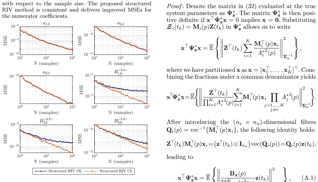
- [Section 6.2, Figures 4 and 5, and Section 4.2, Eq. (37)] The simulation section does not compare the empirical MSE of the estimators against the theoretical covariance P of Eq. (37) or against the CRLB. The paper claims asymptotic efficiency in open loop and minimum covariance among IV estimators in closed loop, but the only evidence provided is that the MSE decays to zero and that the structured estimator has lower variance than the unstructured one. To validate the central efficiency claims, the authors should overlay the theoretical covariance (or the CRLB) on the MSE plots for at least the largest sample sizes, and also verify that the empirical covariance of the estimated parameters approaches P. Without such a comparison, the simulations cannot discriminate between the proposed method's claimed optimality and the mere consistency that any reasonable IV estimator would achieve.
- [Section 5, Theorem 3, and Remark 5] The claim that the closed-loop RIV estimator achieves 'the lower bound on the asymptotic covariance of any instrumental variable method' is stated (after Eq. (41)) with reference to [37,41] and to Theorem 1 of [15], but no proof is given in this manuscript for the additive MIMO case. Since this is one of the two main optimality claims of the paper, the authors should either provide a self-contained proof or explicitly state the precise class of IV estimators over which the lower bound is taken and how the existing SISO/MISO results extend to the present setting. The current statement is too terse for a claim of this strength.
minor comments (5)
- [Section 6.1] There is a typo: 'ranging logarithmically from = 10 3 to N = 105' should read 'from N = 10^3 to N = 10^5'.
- [Section 3, Eqs. (12) and (15)] The notation for the regressor and instrument matrices is dense; it would help to specify the dimensions of each block explicitly, and to state that the operator p in the filter expressions acts on the signal that follows it (as in Remark 1. The current notation may confuse readers who are not already familiar with continuous-time IV methods.
- [Section 4.1, Assumption 4] Assumption 4 (sampling rate) is stated 'for all j >= 1', but the true system parameters and the estimated parameters at each iteration are not known a priori; in practice, this is checked after each iteration. A brief comment on how this assumption is verified in the implementation would improve the presentation.
- [Section 6.2, Figures 4 and 5] The figures would benefit from error bars or shaded confidence regions for the Monte Carlo MSE estimates, and the text should state the number of Monte Carlo runs used for each sample size (M = 300 is given in the setup, but the figures do not indicate variability). This would make the claimed consistency visually harder to dispute.
- [Section 4.2, proof of Theorem 2] The Taylor expansion in Eq. (38) and the subsequent decomposition would be clearer if the authors explicitly stated which terms are op(N) and op(sqrt(N) ||beta_hat - beta*||), and if they numbered the intermediate equalities; the current proof is readable but requires the reader to fill in several standard steps.
Circularity Check
No load-bearing circularity; central asymptotic results are proven from standard IV theory, with self-citations only contextual.
full rationale
The paper's central claims, Theorems 1-3, are derived in the text from the correlation equations (11), the pseudolinear iteration (17), and standard instrumental-variable results ([37], [4], [27]); they are not obtained by fitting to the simulations in Section 6. The instrument matrix (12) is deliberately chosen as a noiseless Jacobian, and the open-loop efficiency result follows by verifying that (37) equals the Fisher information (40), an independent comparison rather than a definitional identity. The closed-loop IV lower bound is attributed to classical references [37,41] with [15] cited as a related additive-SISO case, so no uniqueness theorem is imported from the authors alone. Self-citations [15,45] supply the base algorithm and the ancillary statement that the RIV method minimizes prediction error at convergence; this statement is used only to link (43) to the indirect prediction error method and is not needed to establish Theorem 3's covariance formula. Condition (23) is an explicit, unproven sufficiency condition; it makes Theorem 1 conditional, which is a technical limitation rather than a circular step, since the theorem does not assume the conclusion it purports to prove. The simulations corroborate, but do not define, the theoretical covariance expressions. Therefore no prediction reduces by construction to its inputs.
Assumptions & free parameters
assumptions (9)
- domain assumption Persistency of excitation: input (open loop) or reference (closed loop) is persistently exciting of order at least 2 sum n_i (plus controller order in closed loop).
- domain assumption Quasi-stationarity and statistical independence of input/reference from noise.
- ad hoc to paper At every iteration, estimated denominator polynomials remain stable, coprime with numerators, and (in closed loop) stabilized by the controller.
- domain assumption Sampling frequency exceeds twice the largest imaginary part of the zeros of the product of true and estimated denominators.
- ad hoc to paper The interpolation-error perturbation satisfies inequality (23): ||E{hatPhi Sigma^{-1} Delta_z^T}||_2^2 < sigma_min(E{hatPhi Sigma^{-1} tildePhi_z^T}).
- ad hoc to paper The iterative procedure (17) converges for all sufficiently large N to a solution of the correlation equations.
- domain assumption The mapping f from structured parameters rho to unstructured beta is smooth, injective, and has full-column-rank Jacobian except on a measure-zero set.
- domain assumption Noise v(tk) is i.i.d. Gaussian white for the asymptotic distribution results (Theorems 2 and 3).
- domain assumption The estimated submodel ordering aligns with beta* in Euclidean norm.
Cite this review
Pith. "Pith review of Statistically Optimal Structured Additive MIMO Continuous-time System Identification." pith.science (2026). https://pith.science/paper/7ZL4EPDP
@misc{pith2026250514169,
  author       = {Pith},
  title        = {Pith review of: Statistically Optimal Structured Additive MIMO Continuous-time System Identification},
  year         = {2026},
  howpublished = {\url{https://pith.science/paper/7ZL4EPDP}},
  note         = {Machine review of arXiv:2505.14169}
}
read the original abstract
Many applications in mechanical, acoustic, and electronic engineering require estimating complex dynamical models, often represented as additive multi-input multi-output (MIMO) transfer functions with structural constraints. This paper introduces a two-stage procedure for estimating structured additive MIMO models, where structural constraints are enforced through a weighted nonlinear least-squares projection of the parameter vector initially estimated using a recently developed refined instrumental variables algorithm. The proposed approach is shown to be consistent and asymptotically efficient in open-loop scenarios. In closed-loop settings, it remains consistent despite potential noise model misspecification and achieves minimum covariance among all instrumental variable estimators. Extensive simulations are performed to validate the theoretical findings, and to show the efficacy of the proposed approach.
Figures


Figures from the paper (2 more)

Reference graph
Works this paper leans on
-
[15]
R. A Gonz´ alez, K. Classens, C. R. Rojas, J. S. Welsh, and T. Oomen. Identification of additive continuous-time systems in open and closed loop. Automatica, 173, Article 112013, 2025
work page 2025
-
[1]
M. Akroum and K. Hariche. Extending the SRIV identification algorithm to MIMO LMFD models. Journal of Electrical Engineering and Technology, 4(1):135–142, 2009
work page 2009
-
[2]
R. S. Blom and P.M.J. Van Den Hof. Multivariable frequency domain identification using IV-based linear regression. In Proceedings of the 49th IEEE Conference on Decision and Control, pages 1148–1153, 2010
work page 2010
-
[3]
K. Classens, R. A. Gonz´ alez, and T. Oomen. Recursive Identification of Structured Systems: An Instrumental- Variable Approach Applied to Mechanical Systems.European Journal of Control (in Press) , 2025
work page 2025
- [4]
- [5]
-
[6]
U. Forssell and C.T. Chou. Efficiency of prediction error and instrumental variable methods for closed-loop identification. In Proceedings of the 37th IEEE Conference on Decision and Control, pages 1287–1288, 1998
work page 1998
-
[7]
U. Forssell and L. Ljung. Closed-loop identification revisited. Automatica, 35(7):1215–1241, 1999
work page 1999
Show all 55 references
-
[8]
Garnier, M
H. Garnier, M. Gilson, P. C. Young, and E. Huselstein. An optimal IV technique for identifying continuous-time transfer function model of multiple input systems. Control Engineering Practice, 15(4):471–486, 2007
2007
-
[9]
Garnier and L
H. Garnier and L. Wang (Eds.). Identification of Continuous- time Models from Sampled Data . Springer, 2008
2008
-
[10]
Gawronski
W. Gawronski. Advanced Structural Dynamics and Active Control of Structures . Springer, 2004
2004
-
[11]
Gibson and B
S. Gibson and B. Ninness. Robust maximum-likelihood estimation of multivariable dynamic systems. Automatica, 41(10):1667–1682, 2005
2005
-
[12]
Gilson, H
M. Gilson, H. Garnier, and P.M.J. Van Den Hof. Instrumental variable methods for continuous-time model identification in closed-loop. In Proceedings of the American Control Conference, pages 2846–2851, 2004
2004
-
[13]
Gilson, H
M. Gilson, H. Garnier, P. C. Young, and P. M. J. Van den Hof. Instrumental variable methods for closed-loop continuous- time model identification. In H. Garnier and L. Wang (Eds.). Identification of Continuous-time Models from Sampled Data, pages 133–160. Springer, 2008
2008
-
[14]
Gilson and P.M.J
M. Gilson and P.M.J. Van Den Hof. Instrumental variable methods for closed-loop system identification. Automatica, 41(2):241–249, 2005
2005
-
[16]
A Gonz´ alez, S
R. A Gonz´ alez, S. Pan, C. R. Rojas, and J. S. Welsh. Consistency analysis of refined instrumental variable methods for continuous-time system identification in closed-loop. Automatica, 166, Article 111697, 2024
2024
-
[17]
R. A. Gonz´ alez, C. R. Rojas, S. Pan, and J. S. Welsh. The SRIVC algorithm for continuous-time system identification with arbitrary input excitation in open and closed loop. In 60th IEEE Conference on Decision and Control (CDC) , pages 3004–3009, 2021
2021
-
[18]
R. A. Gonz´ alez, C. R. Rojas, S. Pan, and J. S. Welsh. Parsimonious Identification of Continuous-Time Systems: A Block-Coordinate Descent Approach. IF AC-PapersOnLine, 56(2):4216–4221, 2023
2023
-
[19]
R. A. Gonz´ alez, C. R. Rojas, S. Pan, and J. S. Welsh. Refined instrumental variable methods for unstable continuous-time systems in closed-loop. International Journal of Control , 96(10):2527–2541, 2023
2023
-
[20]
Gourieroux and A
C. Gourieroux and A. Monfort. Statistics and Econometric Models, Volume 1. Cambridge University Press, 1995
1995
-
[21]
He and H
J. He and H. Hjalmarsson. Weighted Null Space Fitting (WNSF): A Link between The Prediction Error Method and Subspace Identification. arXiv preprint arXiv:2411.00506 , 2024
2024 arXiv
-
[22]
Jian, Y.-S
H.-M. Jian, Y.-S. Chen, and M. R. Bai. Acoustic modal analysis of room responses from the perspective of state-space balanced realization with application to field interpolation. The Journal of the Acoustical Society of America, 152(1):240– 250, 2022
2022
-
[23]
Kollar, G
I. Kollar, G. Franklin, and R. Pintelon. On the equivalence of z-domain and s-domain models in system identification. In Instrumentation and Measurement Technology Conference, 1996, volume 1, pages 14–19, 1996
1996
-
[24]
Lange and M
C. Lange and M. Leone. Broadband circuit model for EMI analysis of complex interconnection networks in metallic enclosures of arbitrary shape. IEEE Transactions on Electromagnetic Compatibility, 63(2):474–483, 2020
2020
-
[25]
E. L. Lehmann and G. Casella. Theory of Point Estimation, 2nd ed. Springer, 1998
1998
-
[26]
L. Ljung. Information contents in identification data from closed-loop operation. In Proceedings of 32nd IEEE Conference on Decision and Control, pages 2248–2252, 1993
1993
-
[27]
L. Ljung. System Identification: Theory For The User . Prentice-Hall, second edition, 1999
1999
-
[28]
Ljung, I
L. Ljung, I. Gustavsson, and T. S¨ oderstr¨ om. Identification of linear, multivariable systems operating under linear feedback control. IEEE Transactions on Automatic Control, 19(6):836–840, 1974
1974
-
[29]
Ljung and T
L. Ljung and T. McKelvey. Subspace identification from closed loop data. Signal Processing, 52(2):209–215, 1996. 14
1996
-
[30]
Merc` ere, O
G. Merc` ere, O. Prot, and J. A. Ramos. Identification of parameterized gray-box state-space systems: From a black- box linear time-invariant representation to a structured one. IEEE Transactions on Automatic Control, 59(11):2873–2885, 2014
2014
-
[31]
T. Oomen. Control for precision mechatronics. In Encyclopedia of Systems and Control , pages 267–276. Springer, 2021
2021
-
[32]
S. Pan, R. A. Gonz´ alez, J. S. Welsh, and C. R. Rojas. Consistency analysis of the simplified refined instrumental variable method for continuous-time systems. Automatica, 113, Article 108767, 2020
2020
-
[33]
S. Pan, J. S. Welsh, R. A. Gonz´ alez, and C. R. Rojas. Efficiency analysis of the Simplified Refined Instrumental Variable method for Continuous-time systems. Automatica, 121, Article 109196, 2020
2020
-
[34]
Pintelon and J
R. Pintelon and J. Schoukens. System Identification . John Wiley & Sons, New Jersey, second edition, 2012
2012
-
[35]
H. K. Shirvani, J. Q. C. Zeng, P. Bevers, T. Oomen, and K. Erkorkmaz. Linear time-invariant model identification algorithm for mechatronic systems based on MIMO frequency response data. IEEE/ASME Transactions on Mechatronics, 28(2):703–714, 2023
2023
-
[36]
S¨ oderstr¨ om.Discrete-time Stochastic Systems: Estimation and Control
T. S¨ oderstr¨ om.Discrete-time Stochastic Systems: Estimation and Control. Springer, 2002
2002
-
[37]
S¨ oderstr¨ om and P
T. S¨ oderstr¨ om and P. Stoica.Instrumental Variable Methods for System Identification . Springer, 1983
1983
-
[38]
On the generic consistency of instrumental variable estimates
T S¨ oderstr¨ om and P Stoica. On the generic consistency of instrumental variable estimates. IF AC Proceedings Volumes, 17(2):603–607, 1984
1984
-
[39]
S¨ oderstr¨ om and P
T. S¨ oderstr¨ om and P. Stoica.System Identification. Prentice Hall, 2001
2001
-
[40]
S¨ oderstr¨ om, P
T. S¨ oderstr¨ om, P. Stoica, and B. Friedlander. An Indirect Prediction Error Method for System Identification. Automatica, 27(1):183–188, 1991
1991
-
[41]
S¨ oderstr¨ om, P
T. S¨ oderstr¨ om, P. Stoica, and E. Trulsson. Instrumental variable methods for closed loop systems. IF AC Proceedings Volumes, 20(5):363–368, 1987
1987
-
[42]
V. Solo. Time Series Recursions and Stochastic Approximation. PhD thesis, Australian National University, 1979
1979
-
[43]
P. Tacx, R. Habraken, G. Witvoet, M. Heertjes, and T. Oomen. Identification of an overactuated deformable mirror system with unmeasured outputs. Mechatronics, 99, Article 103158, 2024
2024
-
[44]
P. M. J. Van Den Hof. Closed-loop Issues in system identification. Annual Reviews in Control, 22:173–186, 1998
1998
-
[45]
van der Hulst, R
M. van der Hulst, R. A. Gonz´ alez, K. Classens, N. Dirkx, J. Van De Wijdeven, and T. Oomen. Identification of additive multivariable continuous-time systems. arXiv preprint arXiv:2504.01639, 2025
2025 arXiv
-
[46]
van der Hulst, R
M. van der Hulst, R. A. Gonz´ alez, K. Classens, P. Tacx, N. Dirkx, J. van de Wijdeven, and T. Oomen. Frequency domain identification for multivariable motion control systems: Applied to a prototype wafer stage. arXiv preprint arXiv:2503.02869, 2025
2025 arXiv
-
[47]
A. W. Van der Vaart. Asymptotic Statistics . Cambridge University Press, 2000
2000
-
[48]
Van der Veen, J.-W
G. Van der Veen, J.-W. van Wingerden, M. Bergamasco, M. Lovera, and M. Verhaegen. Closed-loop subspace identification methods: an overview. IET Control Theory & Applications, 7(10):1339–1358, 2013
2013
-
[49]
Vayssettes, G
J. Vayssettes, G. Merc` ere, Y. Bury, and V. Pommier- Budinger. Structured model identification algorithm based on constrained optimisation. In European Control Conference (ECC), pages 1285–1290. IEEE, 2015
2015
-
[50]
Vayssettes, G
J. Vayssettes, G. Merc` ere, P. Vacher, and R. A. De Callafon. Frequency-domain identification of aircraft structural modes from short-duration flight tests. International Journal of Control, 87(7):1352–1372, 7 2014
2014
-
[51]
Voorhoeve, R
R. Voorhoeve, R. De Rozario, W. Aangenent, and T. Oomen. Identifying position-dependent mechanical systems: A modal approach applied to a flexible wafer stage.IEEE Transactions on Control Systems Technology, 29(1):194–206, 2021
2021
-
[52]
P. C. Young and A. Jakeman. Refined instrumental variable methods of recursive time-series analysis. International Journal of Control , 31:741–764, 1980
1980
-
[53]
Zhang and F
M. Zhang and F. Xu. Variational mode decomposition based modal parameter identification in civil engineering. Frontiers of Structural and Civil Engineering , 13:1082–1094, 2019
2019
-
[54]
J. Zhu, J. Ni, and A. J. Shih. Robust machine tool thermal error modeling through thermal mode concept. Journal of Manufacturing Science and Engineering , 130, Article 061006(6), 2008
2008
-
[55]
Zhu and H
Y. Zhu and H. Hjalmarsson. The Box–Jenkins Steiglitz– McBride algorithm. Automatica, 65:170–182, 2016. 15
2016
Reviewed August 7, 2026 · model on record in the stance chip above.
Discussion (0). Continue with ORCID to comment.