Coupling Precipitation Forecasting and Early Warning with Reverse-Martingale Recurrent Neural Networks

Hui-Mean Foo; Yuan-chin Ivan Chang

arxiv: 2607.00331 · v1 · pith:A6L2RLLXnew · submitted 2026-07-01 · 📊 stat.AP

Coupling Precipitation Forecasting and Early Warning with Reverse-Martingale Recurrent Neural Networks

Hui-Mean Foo , Yuan-chin Ivan Chang This is my paper

Pith reviewed 2026-07-02 00:30 UTC · model grok-4.3

classification 📊 stat.AP

keywords precipitation forecastingdrought early warningrecurrent neural networksreverse-martingale penaltychange-point detectionSPI-3 indexhydroclimatic regimesbackward coherence

0 comments

The pith

A recurrent neural network with a reverse-martingale penalty forecasts precipitation as accurately as standard models while turning reconstruction defects into an early drought warning signal.

A machine-rendered reading of the paper's core claim, the machinery that carries it, and where it could break.

The paper seeks to establish that one recurrent model can perform precipitation forecasting and drought early warning simultaneously by adding a backward-coherence penalty. This penalty maintains smoothness of the hidden state when read in reverse time, so the size of the reconstruction defect can feed a sequential change-point detector. A sympathetic reader would care because decisions about water restrictions and drought alerts require noticing when a local regime turns abnormal, something forecast accuracy scores alone do not supply. On daily data from four climates the model matches standard forecast skill and produces steadier states, while the new signal often precedes the operational SPI-3 index.

Core claim

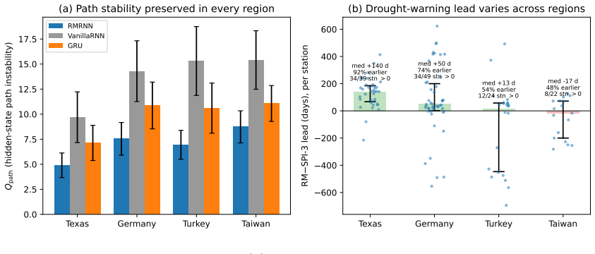
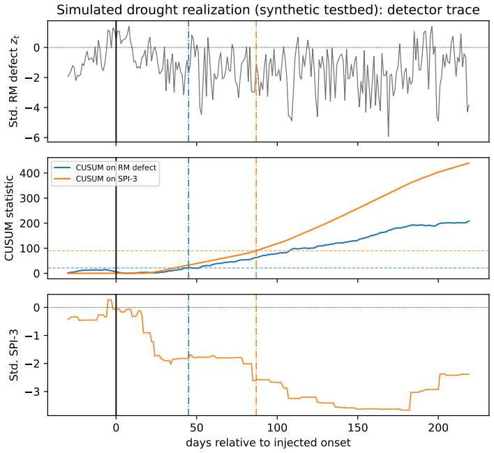
The authors claim that equipping a recurrent network with a reverse-martingale penalty preserves forecast accuracy on real daily precipitation records from monsoonal, semi-arid, temperate, and Mediterranean stations while making the hidden state markedly steadier; the resulting reconstruction defect then functions as an online warning signal that a change-point detector can use to alarm ahead of the SPI-3 index in several regions, with the size of the lead explained by whether drought onset precedes or coincides with the rainfall deficit.

What carries the argument

The reverse-martingale penalty, which enforces backward coherence on the hidden state so that the magnitude of the reconstruction defect becomes the input to a sequential change-point detector for drought onset.

If this is right

Forecast skill remains comparable to a standard recurrent network across all four tested climates.
The hidden state becomes markedly steadier in every region.
The warning signal supplies lead time over the operational SPI-3 index in multiple regions.
The magnitude of the lead varies with the hydroclimatic character of drought onset.
A synthetic study with known onset times supports that the advantage stems from the timing of regime change relative to rainfall deficit.

Where Pith is reading between the lines

These are editorial extensions of the paper, not claims the author makes directly.

The same penalty structure could be applied to other environmental time series where regime shifts precede observable deficits.
Steadier hidden states may reduce error accumulation in multi-step forecasts beyond the horizons tested here.
Extending the detector to temperature or streamflow records would test whether the early-warning benefit generalizes beyond precipitation.

Load-bearing premise

The reconstruction defect produced by the reverse-martingale penalty functions as a reliable indicator of drought regime onset rather than reflecting data properties or detector tuning.

What would settle it

A controlled experiment in which drought onset is forced to coincide exactly with the rainfall deficit in synthetic data with known timing, checking whether the lead-time advantage over SPI-3 disappears.

Figures

Figures reproduced from arXiv: 2607.00331 by Hui-Mean Foo, Yuan-chin Ivan Chang.

**Figure 1.** Figure 1: Real data, four regions. (a) Hidden-state path instability Qpath is reduced by RMRNN relative to the unregularized network in every region (bars are means, error bars ±1 SD across stations; forecast skill preserved, [PITH_FULL_IMAGE:figures/full_fig_p009_1.png] view at source ↗

**Figure 2.** Figure 2: Per-station early-warning lead of the RM-defect CUSUM over the SPI-3 [PITH_FULL_IMAGE:figures/full_fig_p032_2.png] view at source ↗

**Figure 3.** Figure 3: First-alarm day for the RM-defect CUSUM (circles) and the SPI-3 CUSUM [PITH_FULL_IMAGE:figures/full_fig_p033_3.png] view at source ↗

**Figure 4.** Figure 4: Monte-Carlo CUSUM ARL0 calibration on the synthetic testbed, two curves on a single panel: the drought detector (CUSUM on the standardized RM defect) and the heavy-rain detector (CUSUM on precipitation). Empirical ARL0 (reset-on-crossing on a six-year null stream) increases monotonically with the threshold h. Horizontal dotted lines mark the target ARL0 (500 and 1,000); vertical dashed lines mark the calib… view at source ↗

**Figure 5.** Figure 5: One simulated drought realization (synthetic testbed). Top: standardized RM [PITH_FULL_IMAGE:figures/full_fig_p034_5.png] view at source ↗

read the original abstract

Precipitation forecasts are judged by accuracy, but the decisions they support -- when to restrict water, when to warn of drought -- turn on noticing when a local regime is becoming abnormal, which forecast scores alone do not reveal. We ask whether one recurrent model can do both with little or no loss in forecast skill. We add a backward-coherence (reverse-martingale) penalty that keeps the network's hidden state smooth when read backward in time; the size of the resulting reconstruction defect becomes an online warning signal, monitored by a sequential change-point detector. The design is deliberately conservative. On real daily station data from four contrasting climates -- monsoonal Taiwan, semi-arid Texas, temperate Germany, and Mediterranean Anatolia (Turkey) -- the model matches a standard network's forecast skill everywhere, and makes the hidden state markedly steadier in every region. The novelty is the added information: on these real droughts the signal can alarm well ahead of the operational SPI-3 index, giving lead that neither the forecast nor the index provides. This benefit is not uniform across the four regions -- large in one, partial in two others, and near-absent in the fourth. We offer the hydroclimatic character of drought onset, whether it precedes or merely coincides with the rainfall deficit, as a plausible explanation to be tested in future work, supported by a controlled synthetic study with known onset times. The contribution is thus a new and conservative way to read precipitation records: no loss in forecast skill, a steadier model, and an early-warning signal beyond the standard index.

Editorial analysis

A structured set of objections, weighed in public.

Desk editor's note, referee report, simulated authors' rebuttal, and a circularity audit. Tearing a paper down is the easy half of reading it; the pith above is the substance, this is the friction.

Desk Editor's Note private letter to a colleague

The reverse-martingale penalty is a fresh way to turn an RNN's backward coherence into both steadier forecasts and an online drought signal, but the abstract leaves the actual numbers and detector details out so the lead-time claim stays uncheckable.

read the letter

This paper adds a reverse-martingale penalty to a recurrent network so the hidden state stays coherent when read backward; the reconstruction defect then feeds a change-point detector for drought warnings while the main task stays precipitation forecasting.

It does a couple of things cleanly. On daily station data from Taiwan, Texas, Germany, and Turkey the forecast skill stays level with a plain network, and the hidden state becomes noticeably steadier in all four places. The synthetic study with known onset times is a reasonable check on the idea, and the regional variation in warning lead is at least acknowledged rather than glossed over.

The soft spots are the missing pieces that matter most. No exact penalty formula, no detector parameters, no lead-time distributions, and no false-alarm counts appear in what is shown. Without those, it is impossible to tell whether the reported advance over SPI-3 comes from the hydroclimatic timing the authors suggest or from how the detector was set. The non-uniform regional results make the explanation even harder to assess.

This is for people who build or evaluate operational precipitation models and early-warning tools. A reader working on time-series change detection in hydrology would see a concrete new loss term and could judge whether the dual-use framing is worth trying.

I would send it for peer review. The core construction is new and the design stays conservative, so referees can ask for the missing calibration details and the quantitative evidence on lead time.

Referee Report

2 major / 1 minor

Summary. The paper proposes augmenting a recurrent neural network for daily precipitation forecasting with a reverse-martingale penalty on the hidden state to enforce backward coherence. The magnitude of the resulting reconstruction defect is monitored by a sequential change-point detector to generate early-warning signals for drought regime shifts. On real station data from four contrasting climates the model is reported to match a baseline network's forecast skill while producing steadier hidden states and, in some regions, alarms that precede the operational SPI-3 index; a controlled synthetic experiment with known onset times is offered in support.

Significance. If the lead-time claims can be reproduced with full methodological detail, the work would demonstrate a conservative, single-model route to joint forecasting and regime-change detection that adds usable early-warning information beyond standard drought indices without degrading predictive accuracy. The regional heterogeneity and the hydroclimatic interpretation supplied for it would also supply a concrete hypothesis for follow-up studies.

major comments (2)

[Abstract, §3] Abstract and §3 (Methods): the exact functional form of the reverse-martingale penalty, the numerical value of its weight, and the full specification (threshold, window, etc.) of the change-point detector are not supplied. These quantities are load-bearing for the central claim that the reconstruction defect produces verifiable lead time over SPI-3; without them the reported alarms cannot be reproduced or tested for sensitivity to tuning.
[§4] §4 (Results) and synthetic study: no lead-time distributions, false-alarm rates, or statistical significance tests comparing the detector output to SPI-3 onset are presented, nor is an explicit definition of “onset” given for the synthetic case. The non-uniform regional benefit is acknowledged but cannot be attributed to hydroclimatic character versus detector calibration without these quantitative controls.

minor comments (1)

[Abstract] The abstract states that the hidden state is “markedly steadier” but supplies no quantitative metric (e.g., variance of hidden activations or autocorrelation) to support the claim.

Simulated Author's Rebuttal

2 responses · 0 unresolved

We thank the referee for the constructive comments. We address each major point below.

read point-by-point responses

Referee: [Abstract, §3] Abstract and §3 (Methods): the exact functional form of the reverse-martingale penalty, the numerical value of its weight, and the full specification (threshold, window, etc.) of the change-point detector are not supplied. These quantities are load-bearing for the central claim that the reconstruction defect produces verifiable lead time over SPI-3; without them the reported alarms cannot be reproduced or tested for sensitivity to tuning.

Authors: The referee is correct that these details were insufficiently specified in the submitted version. We will revise §3 to supply the exact functional form of the reverse-martingale penalty, the numerical weight used during training, and the complete parameters (threshold, window, etc.) of the change-point detector. The abstract will be updated to reference these additions. revision: yes
Referee: [§4] §4 (Results) and synthetic study: no lead-time distributions, false-alarm rates, or statistical significance tests comparing the detector output to SPI-3 onset are presented, nor is an explicit definition of “onset” given for the synthetic case. The non-uniform regional benefit is acknowledged but cannot be attributed to hydroclimatic character versus detector calibration without these quantitative controls.

Authors: We agree that the current §4 lacks the requested quantitative controls and explicit definitions. The revised manuscript will add lead-time distributions, false-alarm rates, and statistical significance tests comparing detector output to SPI-3. We will also supply an explicit definition of onset for the synthetic experiments. These changes will allow clearer attribution of regional differences. revision: yes

Circularity Check

0 steps flagged

No significant circularity; derivation is self-contained

full rationale

The paper explicitly adds a reverse-martingale penalty term to the training loss to enforce backward smoothness on the hidden state; the resulting reconstruction defect is then fed to an independent sequential change-point detector to produce the warning signal. This is a designed architectural feature, not a quantity that reduces by the model's equations to already-fitted drought labels or forecast targets. No load-bearing self-citation, uniqueness theorem, or fitted-input-renamed-as-prediction appears in the provided abstract or description. The forecast-skill equivalence and lead-time claims are presented as empirical observations on real station data, with the hydroclimatic explanation offered only as a hypothesis for future testing. The central derivation therefore retains independent content and does not collapse to its inputs by construction.

Axiom & Free-Parameter Ledger

2 free parameters · 2 axioms · 1 invented entities

The central claim rests on standard RNN training assumptions plus two new modeling choices (the reverse-martingale penalty and the interpretation of its defect as a drought signal) and at least two tunable components whose values are not reported in the abstract.

free parameters (2)

reverse-martingale penalty weight
The strength of the backward-coherence term must be chosen or cross-validated; its value directly controls both the steadiness of the hidden state and the size of the reconstruction defect used for warning.
change-point detector parameters
Thresholds or window sizes of the sequential change-point detector are required to convert the defect into an alarm; these are not stated and affect reported lead times.

axioms (2)

domain assumption Adding a backward-coherence penalty to an RNN loss preserves forecast skill while producing a usable anomaly signal.
Invoked when the abstract states that forecast skill is maintained everywhere while the hidden state becomes markedly steadier.
ad hoc to paper The reconstruction defect reliably precedes or coincides with drought onset in a manner detectable by a standard change-point method.
The abstract treats the defect size as the warning signal without further justification beyond the synthetic study.

invented entities (1)

reverse-martingale penalty no independent evidence
purpose: Enforce backward coherence in the RNN hidden state so that the resulting reconstruction defect serves as an online drought warning signal.
A new loss term introduced by the paper; no independent evidence outside the four-region experiments and synthetic study is supplied in the abstract.

pith-pipeline@v0.9.1-grok · 5814 in / 1716 out tokens · 34412 ms · 2026-07-02T00:30:50.132509+00:00 · methodology

discussion (0)

Reference graph

Works this paper leans on

27 extracted references · 5 canonical work pages

[1]

and Chen, Y.-L

Chen, C.-S. and Chen, Y.-L. (2003). The rainfall characteristics of Taiwan. Monthly Weather Review,131(7), 1323–1341. doi:https://doi.org/10.1175/ 1520-0493(2003)131%3C1323:TRCOT%3E2.0.CO;2

2003
[2]

J., Hovius, N., Chen, H., Dade, W

Dadson, S. J., Hovius, N., Chen, H., Dade, W. B., Hsieh, M.-L., Willett, S. D., Hu, J.-C., Horng, M.-J., Chen, M.-C., Stark, C. P., Lague, D. and Lin, J.-C. (2003). Linksbetweenerosion, runoffvariabilityandseismicityintheTaiwanorogen.Nature, 426(6967), 648–651. doi:https://doi.org/10.1038/nature02150

work page doi:10.1038/nature02150 2003
[3]

and Milliman, J

Kao, S.-J. and Milliman, J. D. (2008). Water and sediment discharge from small mountainous rivers, Taiwan: The roles of lithology, episodic events, and human activities.The Journal of Geology,116(5), 431–448. doi:https://doi.org/10. 1086/590921

2008
[4]

Vo, T. H. and Liou, Y. A. (2024). Four-decade spring droughts in Taiwan.Journal of Hydrology: Regional Studies,54, Article 101849. doi:https://doi.org/10.1016/ j.ejrh.2024.101849

work page arXiv 2024
[5]

L., 1953:Stochastic Processes

Doob, J. L., 1953:Stochastic Processes. Wiley, 654 pp

1953
[6]

van Merriënboer, C

Cho, K., B. van Merriënboer, C. Gulcehre, D. Bahdanau, F. Bougares, H. Schwenk, and Y. Bengio, 2014: Learning phrase representations using RNN encoder–decoder for statistical machine translation.Proc. 2014 Conf. Empirical Methods in Natural Language Processing, Doha, Qatar, AssociationforComputationalLinguistics, 1724– 1734, doi:10.3115/v1/D14-1179

work page doi:10.3115/v1/d14-1179 2014
[7]

Schmidhuber, 1997: Long short-term memory.Neural Com- put.,9, 1735–1780, doi:10.1162/neco.1997.9.8.1735

Hochreiter, S., and J. Schmidhuber, 1997: Long short-term memory.Neural Com- put.,9, 1735–1780, doi:10.1162/neco.1997.9.8.1735

work page doi:10.1162/neco.1997.9.8.1735 1997
[8]

Commun.,13, 5145

Espeholt, L., and Coauthors, 2022: Deep learning for twelve hour precipitation forecasts.Nat. Commun.,13, 5145

2022
[9]

Data,2, 150066

Funk, C., and Coauthors, 2015: The climate hazards infrared precipitation with stations—a new environmental record for monitoring extremes.Sci. Data,2, 150066

2015
[10]

Žliobait˙ e, A

Gama, J., I. Žliobait˙ e, A. Bifet, M. Pechenizkiy, and A. Bouchachia, 2014: A survey on concept drift adaptation.ACM Comput. Surv.,46(4), Article 44, 37 pp

2014
[11]

Hao, Z., X. Yuan, Y. Xia, F. Hao, and V. P. Singh, 2017: An overview of drought monitoring and prediction systems at regional and global scales.Bull. Amer. Me- teor. Soc.,98, 1879–1896, doi:10.1175/BAMS-D-15-00149.1

work page doi:10.1175/bams-d-15-00149.1 2017
[12]

Hersbach, H., and Coauthors, 2020: The ERA5 global reanalysis.Quart. J. Roy. Me- teor. Soc.,146, 1999–2049. 30

2020
[13]

Constantinou, C

Hundman, K., V. Constantinou, C. Laporte, I. Colwell, and T. Soderstrom, 2018: Detecting spacecraft anomalies using LSTMs and nonparametric dynamic thresh- olding.Proc. 24th ACM SIGKDD, 387–395

2018
[14]

Milly, P. C. D., J. Betancourt, M. Falkenmark, R. M. Hirsch, Z. W. Kundzewicz, D. P. Lettenmaier, and R. J. Stouffer, 2008: Stationarity is dead: Whither water management?Science,319, 573–574

2008
[15]

H., 2005: Orographic precipitation.Annu

Roe, G. H., 2005: Orographic precipitation.Annu. Rev. Earth Planet. Sci.,33, 645–671

2005
[16]

McKee, T. B., N. J. Doesken, and J. Kleist, 1993: The relationship of drought frequency and duration to time scales.Proc. 8th Conf. on Applied Climatology, Ana- heim, CA, AMS, 179–184

1993
[17]

Menne, M. J., I. Durre, R. S. Vose, B. E. Gleason, and T. G. Houston, 2012: An overview of the Global Historical Climatology Network-Daily database.J. At- mos. Oceanic Technol.,29, 897–910

2012
[18]

V., 1986: Optimal stopping times for detecting changes in distri- butions.Ann

Moustakides, G. V., 1986: Optimal stopping times for detecting changes in distri- butions.Ann. Statist.,14, 1379–1387

1986
[19]

Muñoz-Sabater, J., and Coauthors, 2021: ERA5-Land: A state-of-the-art global reanalysis dataset for land applications.Earth Syst. Sci. Data,13, 4349–4383

2021
[20]

Ravuri, S., and Coauthors, 2021: Skilful precipitation nowcasting using deep gener- ative models of radar.Nature,597, 672–677

2021
[21]

Neural Inf

Shi, X., and Coauthors, 2015: Convolutional LSTM network: A machine learning approach for precipitation nowcasting.Adv. Neural Inf. Process. Syst., 802–810

2015
[22]

Sloughter, J. M., A. E. Raftery, T. Gneiting, and C. Fraley, 2007: Probabilistic quan- titative precipitation forecasting using Bayesian model averaging.Mon. Wea. Rev., 135, 3209–3220

2007
[23]

Wang, Y., M. Long, J. Wang, Z. Gao, and P. S. Yu, 2017: PredRNN: Recurrent neural networks for predictive learning using spatiotemporal LSTMs.Adv. Neural Inf. Process. Syst., 879–888

2017
[24]

World Meteorological Organization, 2012: Standardized Precipitation Index User Guide. WMO-No. 1090, 24 pp

2012
[25]

N., 1969: The predictability of a flow which possesses many scales of motion.Tellus,21, 289–307

Lorenz, E. N., 1969: The predictability of a flow which possesses many scales of motion.Tellus,21, 289–307

1969
[26]

F., and M

Ropelewski, C. F., and M. S. Halpert, 1987: Global and regional scale precipitation patterns associated with the El Niño/Southern Oscillation.Mon. Wea. Rev.,115, 1606–1626

1987
[27]

Wu, and K.-M

Wang, B., R. Wu, and K.-M. Lau, 2001: Interannual variability of the Asian summer monsoon: contrasts between the Indian and the western North Pacific–East Asian monsoons.J. Climate,14, 4073–4090. 31 120.00 120.25 120.50 120.75 121.00 121.25 121.50 121.75 122.00 Longitude (°E) 22.0 22.5 23.0 23.5 24.0 24.5 25.0Latitude (°N) 2020 21 T aiwan drought: 22 CWA ...

2001

[1] [1]

and Chen, Y.-L

Chen, C.-S. and Chen, Y.-L. (2003). The rainfall characteristics of Taiwan. Monthly Weather Review,131(7), 1323–1341. doi:https://doi.org/10.1175/ 1520-0493(2003)131%3C1323:TRCOT%3E2.0.CO;2

2003

[2] [2]

J., Hovius, N., Chen, H., Dade, W

Dadson, S. J., Hovius, N., Chen, H., Dade, W. B., Hsieh, M.-L., Willett, S. D., Hu, J.-C., Horng, M.-J., Chen, M.-C., Stark, C. P., Lague, D. and Lin, J.-C. (2003). Linksbetweenerosion, runoffvariabilityandseismicityintheTaiwanorogen.Nature, 426(6967), 648–651. doi:https://doi.org/10.1038/nature02150

work page doi:10.1038/nature02150 2003

[3] [3]

and Milliman, J

Kao, S.-J. and Milliman, J. D. (2008). Water and sediment discharge from small mountainous rivers, Taiwan: The roles of lithology, episodic events, and human activities.The Journal of Geology,116(5), 431–448. doi:https://doi.org/10. 1086/590921

2008

[4] [4]

Vo, T. H. and Liou, Y. A. (2024). Four-decade spring droughts in Taiwan.Journal of Hydrology: Regional Studies,54, Article 101849. doi:https://doi.org/10.1016/ j.ejrh.2024.101849

work page arXiv 2024

[5] [5]

L., 1953:Stochastic Processes

Doob, J. L., 1953:Stochastic Processes. Wiley, 654 pp

1953

[6] [6]

van Merriënboer, C

Cho, K., B. van Merriënboer, C. Gulcehre, D. Bahdanau, F. Bougares, H. Schwenk, and Y. Bengio, 2014: Learning phrase representations using RNN encoder–decoder for statistical machine translation.Proc. 2014 Conf. Empirical Methods in Natural Language Processing, Doha, Qatar, AssociationforComputationalLinguistics, 1724– 1734, doi:10.3115/v1/D14-1179

work page doi:10.3115/v1/d14-1179 2014

[7] [7]

Schmidhuber, 1997: Long short-term memory.Neural Com- put.,9, 1735–1780, doi:10.1162/neco.1997.9.8.1735

Hochreiter, S., and J. Schmidhuber, 1997: Long short-term memory.Neural Com- put.,9, 1735–1780, doi:10.1162/neco.1997.9.8.1735

work page doi:10.1162/neco.1997.9.8.1735 1997

[8] [8]

Commun.,13, 5145

Espeholt, L., and Coauthors, 2022: Deep learning for twelve hour precipitation forecasts.Nat. Commun.,13, 5145

2022

[9] [9]

Data,2, 150066

Funk, C., and Coauthors, 2015: The climate hazards infrared precipitation with stations—a new environmental record for monitoring extremes.Sci. Data,2, 150066

2015

[10] [10]

Žliobait˙ e, A

Gama, J., I. Žliobait˙ e, A. Bifet, M. Pechenizkiy, and A. Bouchachia, 2014: A survey on concept drift adaptation.ACM Comput. Surv.,46(4), Article 44, 37 pp

2014

[11] [11]

Hao, Z., X. Yuan, Y. Xia, F. Hao, and V. P. Singh, 2017: An overview of drought monitoring and prediction systems at regional and global scales.Bull. Amer. Me- teor. Soc.,98, 1879–1896, doi:10.1175/BAMS-D-15-00149.1

work page doi:10.1175/bams-d-15-00149.1 2017

[12] [12]

Hersbach, H., and Coauthors, 2020: The ERA5 global reanalysis.Quart. J. Roy. Me- teor. Soc.,146, 1999–2049. 30

2020

[13] [13]

Constantinou, C

Hundman, K., V. Constantinou, C. Laporte, I. Colwell, and T. Soderstrom, 2018: Detecting spacecraft anomalies using LSTMs and nonparametric dynamic thresh- olding.Proc. 24th ACM SIGKDD, 387–395

2018

[14] [14]

Milly, P. C. D., J. Betancourt, M. Falkenmark, R. M. Hirsch, Z. W. Kundzewicz, D. P. Lettenmaier, and R. J. Stouffer, 2008: Stationarity is dead: Whither water management?Science,319, 573–574

2008

[15] [15]

H., 2005: Orographic precipitation.Annu

Roe, G. H., 2005: Orographic precipitation.Annu. Rev. Earth Planet. Sci.,33, 645–671

2005

[16] [16]

McKee, T. B., N. J. Doesken, and J. Kleist, 1993: The relationship of drought frequency and duration to time scales.Proc. 8th Conf. on Applied Climatology, Ana- heim, CA, AMS, 179–184

1993

[17] [17]

Menne, M. J., I. Durre, R. S. Vose, B. E. Gleason, and T. G. Houston, 2012: An overview of the Global Historical Climatology Network-Daily database.J. At- mos. Oceanic Technol.,29, 897–910

2012

[18] [18]

V., 1986: Optimal stopping times for detecting changes in distri- butions.Ann

Moustakides, G. V., 1986: Optimal stopping times for detecting changes in distri- butions.Ann. Statist.,14, 1379–1387

1986

[19] [19]

Muñoz-Sabater, J., and Coauthors, 2021: ERA5-Land: A state-of-the-art global reanalysis dataset for land applications.Earth Syst. Sci. Data,13, 4349–4383

2021

[20] [20]

Ravuri, S., and Coauthors, 2021: Skilful precipitation nowcasting using deep gener- ative models of radar.Nature,597, 672–677

2021

[21] [21]

Neural Inf

Shi, X., and Coauthors, 2015: Convolutional LSTM network: A machine learning approach for precipitation nowcasting.Adv. Neural Inf. Process. Syst., 802–810

2015

[22] [22]

Sloughter, J. M., A. E. Raftery, T. Gneiting, and C. Fraley, 2007: Probabilistic quan- titative precipitation forecasting using Bayesian model averaging.Mon. Wea. Rev., 135, 3209–3220

2007

[23] [23]

Wang, Y., M. Long, J. Wang, Z. Gao, and P. S. Yu, 2017: PredRNN: Recurrent neural networks for predictive learning using spatiotemporal LSTMs.Adv. Neural Inf. Process. Syst., 879–888

2017

[24] [24]

World Meteorological Organization, 2012: Standardized Precipitation Index User Guide. WMO-No. 1090, 24 pp

2012

[25] [25]

N., 1969: The predictability of a flow which possesses many scales of motion.Tellus,21, 289–307

Lorenz, E. N., 1969: The predictability of a flow which possesses many scales of motion.Tellus,21, 289–307

1969

[26] [26]

F., and M

Ropelewski, C. F., and M. S. Halpert, 1987: Global and regional scale precipitation patterns associated with the El Niño/Southern Oscillation.Mon. Wea. Rev.,115, 1606–1626

1987

[27] [27]

Wu, and K.-M

Wang, B., R. Wu, and K.-M. Lau, 2001: Interannual variability of the Asian summer monsoon: contrasts between the Indian and the western North Pacific–East Asian monsoons.J. Climate,14, 4073–4090. 31 120.00 120.25 120.50 120.75 121.00 121.25 121.50 121.75 122.00 Longitude (°E) 22.0 22.5 23.0 23.5 24.0 24.5 25.0Latitude (°N) 2020 21 T aiwan drought: 22 CWA ...

2001