REVIEW 1 major objections 7 minor
$\mathrm{L}^p$ bounds for parabolic Riesz transforms with rough coefficients: The case $1<p \leq 2$
T0 review · 1 major / 7 minor · reviewed 2026-07-08 · glm-5.2
Pith's one-line read Parabolic Riesz transforms bounded on L^p with rough coefficients
desk verdict First L^p bounds for parabolic Riesz transforms with non-autonomous measurable coefficients; the dual-geometry off-diagonal framework is the real innovation. read the letter →
The pith
A machine-rendered reading of the paper's core claim, the machinery that carries it, and where it could break.
The reading
What carries the argument
Space-time off-diagonal estimates combining parabolic cubes (small scale) with time-stretched annuli modeled on Bessel kernel level sets (large scale); Blunck-Kunstmann extrapolation adapted to two incompatible geometries; iterative bootstrap along parabolic Sobolev conjugates; commutator identity [H*, η] = -(∂_t η) enabling local splitting of temporal off-diagonal estimates
What would settle it
Construct a bounded measurable elliptic coefficient A in dimension n ≥ 2 for which p_-(H) is strictly below 2★, or show that in dimension n = 1, p_-(H) = 1 fails for some complex coefficient.
Extended reading notes
Core claim
The critical exponent p_-(H) governing L^p boundedness of the parabolic Riesz transform equals q_-(H) and lies in [1, 2★), and this range is sharp. The identification rests on a two-geometry off-diagonal framework: parabolic cubes for small scales and time-stretched annuli for large scales, which together convert spatial exponential decay into sufficient temporal decay. A bootstrap argument along parabolic Sobolev conjugates then iteratively extends the boundedness range from L^2 down to (p_-(H), 2], with each extrapolation step's interval independent of the starting exponent. For real coefficients, Gaussian heat kernel bounds force p_-(H) = 1, and the spatial gradient component achieves the
Load-bearing premise
The off-diagonal estimates for temporal supports rely on the commutator [H*, η] = -(∂_t η) being a local multiplication operator, which allows the dual estimate to split into local and non-local terms and ultimately controls the decay rate. If this commutator structure were lost — for instance, under a different operator realization or with lower regularity — the off-diagonal framework and the bootstrap argument would fail.
Editorial extensions
If this is right
- The two-geometry off-diagonal framework may extend to other non-local operators where a single metric cannot capture both local and large-scale behavior, such as generalized Stokes operators.
- The p-sensitivity of the off-diagonal decay rate (ε = 1 + 1/(1+p')) suggests that coefficient-dependent lower bounds on p_-(H) could be computed for specific operator classes.
- The sharpness construction via Mooney's irregular solutions in dimension n ≥ 2 raises the question of whether p_-(H) = 1 always holds in dimension n = 1, which remains open.
- The weak type (1,1) bound for the spatial gradient component with real coefficients leaves open whether the full Riesz transform including D_t^{1/2} H^{-1/2} also satisfies this endpoint estimate.
- The extrapolation range for p > 2 is conjectured to be governed by a dual critical exponent q_+(H), analogous to the elliptic setting, but duality cannot be directly applied due to the limited-range phenomenon.
Reading between the lines
- The two-geometry strategy may apply more broadly to operators where a non-local component (here D_t^{1/2}) couples variables in a way that destroys single-metric structure, suggesting a general principle: when kernel decay is insufficient in one variable, a change of geometry can trade decay from another variable to compensate.
- The sharpness result in n ≥ 2 but not n = 1 hints that the obstruction to p_-(H) = 1 is fundamentally tied to spatial dimension, possibly reflecting the interplay between the parabolic scaling dimension n+2 and the singularity structure of irregular solutions.
- The commutator identity [H*, η] = -(∂_t η) being a local multiplication operator is the structural linchpin; if this locality were lost under different operator realizations or lower regularity, the entire off-diagonal and bootstrap framework would fail, suggesting that the result's reach depends on preserving this commutator structure.
Editorial analysis
A structured set of objections, weighed in public.
Referee Report
Summary. This paper establishes L^p bounds for parabolic Riesz transforms R_H = D H^{-1/2} associated with non-autonomous second-order parabolic operators H = ∂_t − div_x(A∇_x) with bounded measurable coefficients on R^{n+1}. The main result (Theorem 1.3) identifies the maximal open range (p_-(H), 2] for L^p boundedness, where p_-(H) = q_-(H) ∈ [1, 2★) with 2★ = 2(n+2)/(n+4). For real coefficients, p_-(H) = 1 and the spatial component ∇_x H^{-1/2} is weak type (1,1). The range is shown to be sharp for n ≥ 2. The proof combines novel space-time off-diagonal estimates (Section 4) exploiting two complementary geometries—parabolic cubes on small scales and time-stretched annuli on large scales—with a Blunck–Kunstmann-type extrapolation framework (Section 5) and a bootstrap argument (Section 6) identifying p_-(H) = q_-(H).
Significance. This is a substantial contribution to the limited-range extrapolation theory for Riesz transforms with rough coefficients. The key technical innovation is the space-time off-diagonal framework of Section 4, where the commutator locality [H*, η] = −(∂_t η) (Proposition 4.4) is leveraged to convert spatial exponential decay into temporal algebraic decay with a p-sensitive exponent ε = 1 + 1/(1+p') > 1. The dual geometry (parabolic cubes vs. time-stretched annuli) is a genuine new idea that falls outside standard Calderón–Zygmund theory on spaces of homogeneous type. The sharpness result (Section 9) via Mooney's irregular solutions provides a falsifiable endpoint. The identification p_-(H) = q_-(H) via the bootstrap in Theorem 6.1, together with the iterative extrapolation in Theorem 7.3, constitutes the central achievement. The paper builds on the L^2 theory of [1, 9] and resolvent bounds of [1] as external inputs.
major comments (1)
- The stress-test concern regarding the Jensen step in (4.7) at the endpoint p = 1 does not, on careful reading, create a gap in the complex-coefficient case. Proposition 4.4 is stated for p ∈ (1, 2], and the exponent ε = 1 + 1/(1+p') is strictly greater than 1 for all such p. The bootstrap in Theorem 6.1, Step 2 constructs a decreasing sequence s_n → p where p > p_-(H) is fixed but arbitrary. Since p_-(H) ≥ 1 for complex coefficients and the bootstrap only needs to approach p > p_-(H) ≥ 1, the sequence s_n stays bounded away from 1 whenever p > 1. The case p_-(H) = 1 is handled separately in Section 8 via Gaussian bounds, bypassing the bootstrap entirely. The concern is well-raised but ultimately does not land: the paper's architecture correctly separates the complex-coefficient bootstrap (which never needs p = 1) from the real-coefficient case (which uses a different mechanism). I have a
minor comments (7)
- Section 5.1 title: 'Exrapolation' should read 'Extrapolation'.
- Proof of Theorem 8.5: 'we imnose' should be 'we impose'.
- In the proof of Proposition 4.4, the transition from the dual estimate to the primal estimate via duality is stated briefly. A one-line clarification that the L^{p'} bound for (λ E*_λ D^{1/2}_t) transfers to the L^p bound for (λ D^{1/2}_t E_λ) by duality would improve readability.
- The notation 2★ is used before its definition in the statement of Theorem 1.3. Moving the definition 2★ = 2(n+2)/(n+4) to appear before part (1) of the theorem would help the reader.
- In the proof of Theorem 7.3, the condition 3α ≥ β + 1 is imposed mid-proof. A brief remark explaining the role of this condition (ensuring sufficient decay in the functional calculus) would aid the reader.
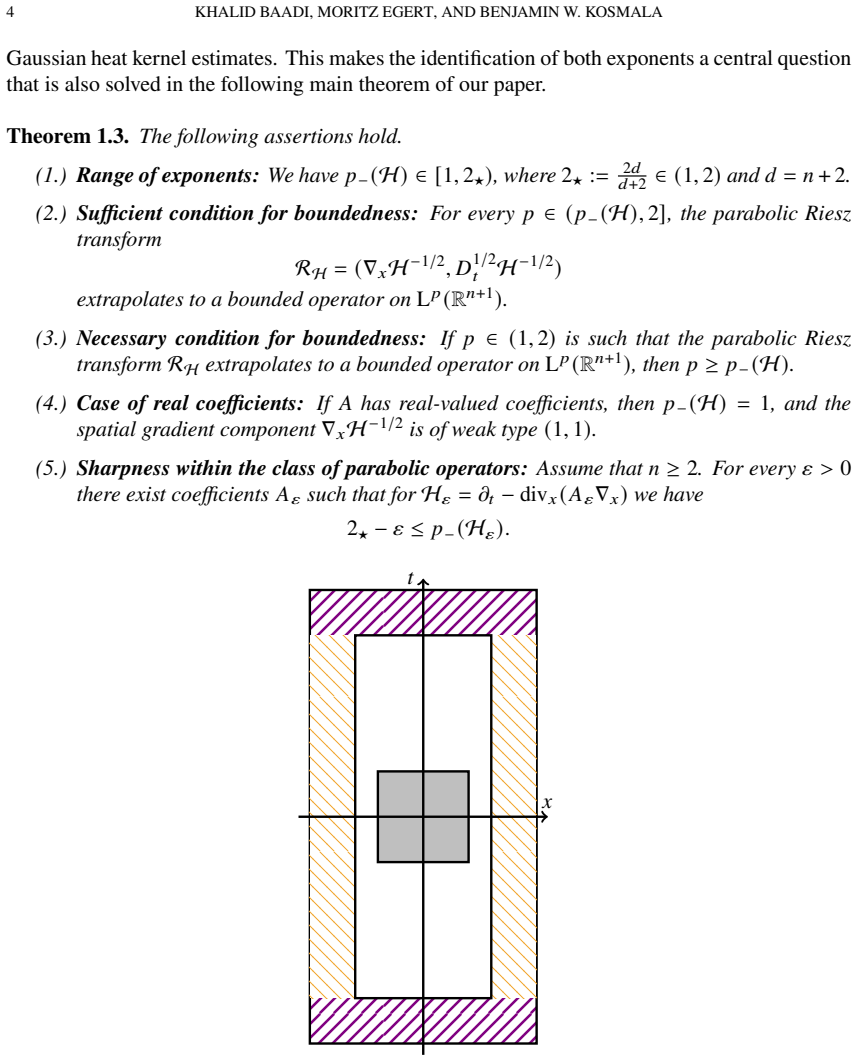
- Figure 1: the caption mentions 'typically N ≥ 2^n' but the role of N in controlling the kernel decay via (1.2) could be stated more explicitly. A brief sentence connecting N to the requirement ε > 1 on the full annulus would avoid confusion.
- In Lemma 7.5, the exponents ϱ_1, ϱ_2 are introduced but their relationship to p_-(H) could be stated more explicitly. Clarifying that ϱ_1, ϱ_2 ∈ (p_-(H), p) would improve clarity.
Simulated Author's Rebuttal
We thank the referee for the careful reading and the positive assessment. The referee raises a single major comment concerning a potential stress-test of the Jensen step in (4.7) at the endpoint p=1 in the complex-coefficient case. As we explain below, we agree with the referee's analysis that no gap exists: the architecture of the paper correctly separates the complex-coefficient bootstrap (which operates strictly for p>1) from the real-coefficient case (which uses Gaussian bounds and a different mechanism).
read point-by-point responses
-
Referee: The stress-test concern regarding the Jensen step in (4.7) at the endpoint p = 1 does not, on careful reading, create a gap in the complex-coefficient case. Proposition 4.4 is stated for p in (1,2], and the exponent epsilon = 1 + 1/(1+p') is strictly greater than 1 for all such p. The bootstrap in Theorem 6.1, Step 2 constructs a decreasing sequence s_n to p where p > p_-(H) is fixed but arbitrary. Since p_-(H) >= 1 for complex coefficients and the bootstrap only needs to approach p > p_-(H) >= 1, the sequence s_n stays bounded away from 1 whenever p > 1. The case p_-(H) = 1 is handled separately in Section 8 via Gaussian bounds, bypassing the bootstrap entirely. The concern is well-raised but ultimately does not land: the paper's architecture correctly separates the complex-coefficient bootstrap (which never needs p = 1) from the real-coefficient case (which uses a different mechanism).
Authors: We thank the referee for the careful and precise analysis of this point. We agree entirely with the assessment. To confirm the referee's reasoning explicitly: Proposition 4.4 is stated for p in (1,2], and the exponent epsilon = 1 + 1/(1+p') satisfies epsilon > 1 for all such p, tending to 1 only in the limit as p tends to 1. In the bootstrap of Theorem 6.1, Step 2, one fixes an arbitrary p in (p_-(H), 2] and constructs a decreasing sequence (s_n) converging to p. Since p > p_-(H) >= 1, the sequence s_n remains bounded away from 1, and thus epsilon evaluated at s_n remains strictly greater than 1 throughout the iteration. The Jensen step in (4.7) is therefore always applied with p' finite. The endpoint p_-(H) = 1 for real coefficients is treated in Section 8 via Gaussian kernel bounds (Lemma 8.2), which bypasses the bootstrap and the p-sensitive off-diagonal estimates of Section 4 entirely. No revision to the mathematical content is needed. We will add a brief clarifying remark in the text near the statement of Proposition 4.4 or in the proof of Theorem 6.1, Step 2, explicitly noting that the bootstrap sequence stays bounded away from p=1 whenever p > p_-(H) >= 1, so that epsilon > 1 is maintained throughout. This should preempt any reader having the same well-motivated concern. revision: partial
Circularity Check
No circularity found: the derivation chain is self-contained with external foundations
full rationale
The paper's main derivation chain proceeds as follows: (1) The L^2 theory (Theorem 2.3) is imported from [1, 9] — these are the parabolic Kato square root estimates, major independent results with their own complete proofs. While Egert is a co-author of both this paper and [1]/[9], the cited results are not assumptions of the present paper's conclusions; they are the L^2 starting point from which extrapolation proceeds. (2) The space-time off-diagonal estimates (Proposition 4.4, Theorem 4.10) are genuinely derived from the commutator identity [H*, η] = -(∂_t η) and a Jensen inequality step, yielding the exponent ε = 1 + 1/(1+p') by optimizing γ in (4.8). No input is renamed as a prediction. (3) The extrapolation framework (Theorem 5.1, Proposition 5.10) consists of general harmonic analysis criteria attributed to Blunck–Kunstmann [21] and inspired by [40, 18]; these are abstract tools not specific to this paper's operators. (4) The bootstrap in Theorem 6.1 proving p_-(H) = q_-(H) starts from L^2 boundedness and iterates downward using the off-diagonal estimates at each current exponent s_n, not at the target p — this is a genuine bootstrap, not a definitional identity. (5) The sufficient condition (Theorem 7.3) and necessary condition (Proposition 7.12) together form a two-sided characterization, each with independent proofs. (6) The sharpness result (Section 9) uses Mooney's construction [42], an external result. The self-citations to [1, 7, 9] are for foundational results with independent proofs that do not assume the conclusions of this paper. No step reduces to its inputs by construction.
Assumptions & free parameters
free parameters (4)
- N (stretching parameter) =
N ≥ 4, chosen sufficiently large
- α (functional calculus parameter) =
α ≥ 2N+1, chosen sufficiently large
- β (resolvent power) =
β ≥ 1, integer, chosen via Lemma 7.5
- M, κ (ellipticity constants) =
Input from the coefficient class (2.2)
assumptions (5)
- domain assumption The maximal restriction of H to L^2(R^{n+1}) is m-accretive and injective, with domain of its square root equal to the energy space E (Theorem 2.3, from [1, 9]).
- domain assumption The commutator [H*, η] = −(∂_t η) is a local multiplication operator for η ∈ C_b^∞(R) acting in the t-variable (proof of Proposition 4.4, Section 4.1).
- domain assumption Gaussian upper bounds for the heat kernel are available when A has real coefficients (Lemma 8.2, from [8]).
- domain assumption Mooney's irregular weak solutions to uniformly parabolic equations exist with the stated pointwise bounds (Section 9, from [42]).
- standard math The Marcinkiewicz multiplier theorem applies to the multiplier m = (iτ + |ξ|²)^{1/2}/(|τ|^{1/2} + i|ξ|) on R^{n+1} (Appendix A, from [34]).
Cite this review
Pith. "Pith review of $\mathrm{L}^p$ bounds for parabolic Riesz transforms with rough coefficients: The case $1<p \leq 2$." pith.science (2026). https://pith.science/paper/AJQ4LJGA
@misc{pith2026260705181,
  author       = {Pith},
  title        = {Pith review of: $\mathrmL^p$ bounds for parabolic Riesz transforms with rough coefficients: The case $1<p \leq 2$},
  year         = {2026},
  howpublished = {\url{https://pith.science/paper/AJQ4LJGA}},
  note         = {Machine review of arXiv:2607.05181}
}
abstract
We establish the first results on $\mathrm{L}^p$ bounds for Riesz transforms associated with non-autonomous second order parabolic differential operators in divergence form with bounded coefficients that depend measurably on all variables. In the case of complex coefficients, we identify the maximal open range of exponents $1<p \leq2$ through the availability of $\mathrm{L}^p$ resolvent bounds. This open range always contains the lower parabolic Sobolev conjugate of $2$ and the result is sharp in spatial dimension $n \geq 2$. For real coefficients, we prove extrapolation to the full range. Our argument relies on novel space-time off-diagonal bounds based on two complementary geometries: parabolic cubes on small scales and regions modeled after the half-order time derivative of a parabolic Bessel potential on large scales.
Figures


Figures from the paper (1 more)

Reviewed July 8, 2026 · model on record in the stance chip above.
Discussion (0). Continue with ORCID to comment.