REVIEW 3 major objections 4 minor 70 references
A multispectral analysis of the northeastern shell of IC 443
T0 review · 3 major / 4 minor · reviewed 2026-08-14 · deepseek-v4-flash
Pith's one-line read The northeastern shell of IC 443 can be explained by one near-solar abundance recipe combined with shocks of different velocity, density, and recombination age, not by spatially varying chemistry.
desk verdict A useful new SITELLE dataset and a clever two-shock grid, but the paper's own 45% fit success undermines the claim that one abundance set is sufficient. read the letter →
The pith
A machine-rendered reading of the paper's core claim, the machinery that carries it, and where it could break.
The reading
What carries the argument
The load-bearing object is the radiative-shock model grid computed with a standard shock-physics code, parameterized by shock velocity, pre-shock density, cut-off temperature (the temperature at which a shock's recombination zone is truncated, standing in for shock age or completeness), and a fixed transverse magnetic field of $B_0 = 1$ microgauss. Two model-building choices carry the argument: first, [O III]/[O II], [O III]/Hβ, and [S II]/Hα ratios are read as diagnostics of shock velocity and age; second, since observed filaments cross on the line of sight, pairs of models are summed according to the binomial coefficient $C(n,r)$ with $r=2$, producing 1.6 billion two-shock combinations that are compared with every observed spectrum. The cut-off temperature is what lets 'incomplete' shocks—those not yet fully recombined—explain the high [O III]/Hβ ratios that complete models cannot.
What would settle it
Measure the magnetic field in the northeastern shell—for example from Faraday rotation of background polarized sources or Zeeman splitting in the associated molecular gas—and recompute the model grid with the measured field. If a field of several microgauss or compressed 10 microgauss fields in radiative shocks still allows the quoted 20–60 cm$^{-3}$ densities and 75 km/s peak, the conclusion stands; if not, the inferred shock conditions are an artifact of the assumed field.
Extended reading notes
Core claim
On its own terms, the paper establishes that the northeastern shell of IC 443 is not chemically patchy: a single set of abundances close to solar values, combined with varying shock velocity, pre-shock density, and shock maturity, reproduces the measured line-intensity ratios. This conclusion rests on a grid of 57,032 shock models spanning velocities 20–150 km s$^{-1}$, pre-shock densities 14–60 cm$^{-3}$, and cut-off temperatures 1000–20,000 K, with a fixed magnetic field of 1 microgauss. Because single shock models fail for many spectra, pairs of shock models were summed: of 35,479 observed spectra, about 45% matched to within 5% in all ten line ratios, and the surviving 16,215 models favor shock velocities around 75 km s$^{-1}$, lower pre-shock densities around 20 cm$^{-3}$, and a spread of recombination stages. The paper also resolves, even at modest spectral resolution, approaching and receding velocity components whose honeycomb versus smooth morphologies imply different interstellar-medium conditions on the two sides of the shell.
Load-bearing premise
The argument assumes the magnetic field is a constant $B_0 = 1$ microgauss throughout IC 443, a value the paper adopts without measuring it; if the real field is stronger, the inferred pre-shock densities and fitted shock models shift.
Editorial extensions
If this is right
- The optical line-ratio maps of the northeastern shell can be read as maps of shock velocity, pre-shock density, and recombination age rather than maps of abundance.
- If line-of-sight pairs of shocks are required for many spectra, single-component interpretations of IC 443 filaments are incomplete, and future work should treat overlapping components as the norm.
- The 75 km s$^{-1}$ preferred velocity and 20–60 cm$^{-3}$ densities anchor where the blast wave is in its evolution against the atomic medium.
- The distinct morphologies of the approaching and receding components mean the shell is encountering different interstellar-medium conditions on its near and far sides, which future higher-resolution cubes could quantify.
- High [N II]/Hα regions without [O III] are consistent with slow shocks and possibly localized nitrogen enhancement, an exception to the single-abundance rule that the paper identifies but cannot fully constrain.
Reading between the lines
- If the single-abundance claim extends to the rest of IC 443, the X-ray-derived abundance enhancements reported for other parts of the remnant may be confined to isolated ejecta knots rather than distributed throughout the shell; optical ratio maps alone would then overstate chemical mixing.
- The same two-shock summation procedure could be applied to other mixed-morphology remnants with multiple velocity components, where degeneracies will need to be broken by independent measures such as Balmer-line widths or magnetic field strengths.
- The fixed 1 microgauss field is the main lever on the quoted density range; re-running the grid with fields of a few microgauss, as expected in compressed radiative shocks, would test whether the 20–60 cm$^{-3}$ range is robust.
- The dip in the velocity histogram at 75 km s$^{-1}$ arises from the steep [O III]/[O II] ratio there; combining the line-ratio method with proper-motion or Balmer-width estimates would check whether the peak is real or an artifact of this sensitivity.
Signed reviews
Editorial analysis
A structured set of objections, weighed in public.
Referee Report
Summary. The paper presents optical multispectral observations of the northeastern shell of supernova remnant IC 443 using the SITELLE imaging Fourier transform spectrometer. Three spectral cubes provide maps of nine emission lines over an 11'x11' field. The authors construct line-ratio maps, correct for extinction using Halpha/Hbeta (E(B-V)=0.8-1.1), and derive electron densities from [SII] (100-2500 cm^-3). They compare the observed ratios with a grid of 57,032 MAPPINGS V shock models, including truncated shocks, and with linear combinations of two shock models. They infer shock velocities of 20-150 km/s (most common 75 km/s), pre-shock densities of 20-60 cm^-3, and shocks at various recombination stages. The central claim is that a single set of near-solar abundances combined with varying shock parameters is sufficient to explain the measured line ratios. The paper also separates red- and blue-shifted velocity components of the nebula, finding morphological differences.
Significance. If the modeling conclusions hold, this study would demonstrate that a single abundance set with two-component shock summation can explain most of the observed line-ratio variability in a complex SNR, which would be a valuable step forward. The observational products—extinction-corrected line ratio maps, electron density maps, and the kinematic separation—are well founded and will be useful for the community. The paper is transparent about its model-fitting procedure, including the grid parameters and the 5% matching criterion. However, the modeling is weakened by the tuning of nitrogen and sulphur abundances to the same data used for validation, and by the reported 45% fit fraction, which directly limits the strength of the 'sufficient abundances' claim. The large grid and the explicit statement of the matching criterion are commendable, as is the clear documentation of the model-fitting procedure.
major comments (3)
- [Section 3.3 and Section 5 (v)] The statement that a single set of abundances is sufficient to explain the measured ratios is not supported by the quantitative results. Only 45% of the 35,479 selected spectra are fitted by any two-shock combination within the 5% tolerance on all 10 line-ratio diagrams; the remaining 55% are unexplained. The text acknowledges this (Section 3.3, 'about 45% of the selected spectra were fitted') and attributes the gap to 'one or more than three components,' but no test is provided for that hypothesis. Section 5 (v) should be rephrased to state that the single-abundance, two-shock framework can account for a subset of the observed spectra, or the analysis should be extended to test whether additional components actually close the gap.
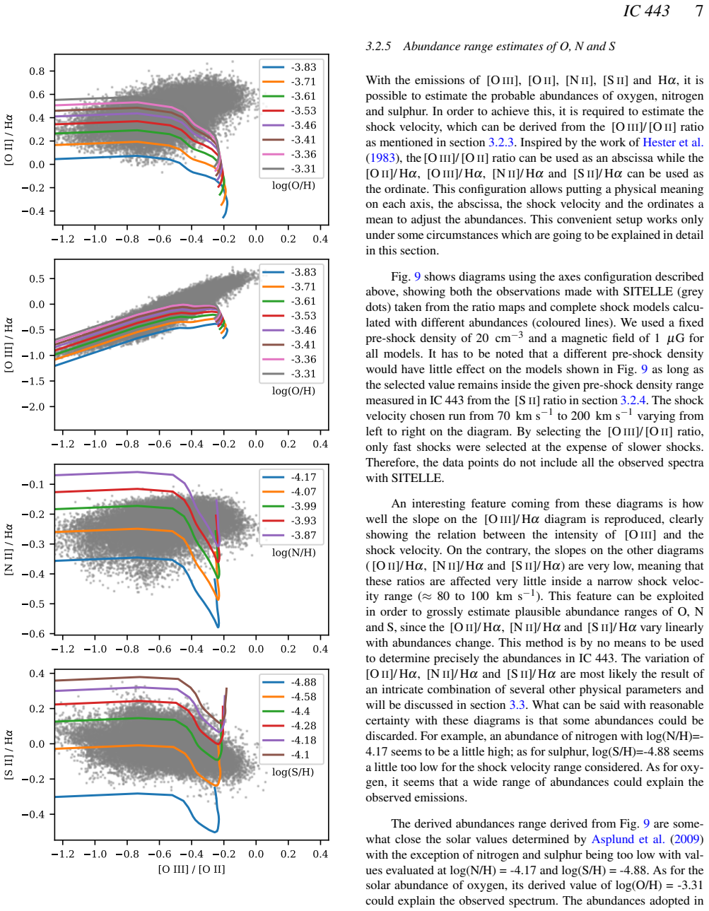
- [Section 3.2.5 and Table 2] The nitrogen and sulphur abundances are chosen by allowing the model curves to pass through the observed point cloud in Fig. 9, and the same abundances are then used in the Section 3.3 grid that forms the basis of the 'single set of abundances is sufficient' conclusion. This is circular to the extent that the abundance set is tuned to the same data used for the validation. Even though the authors caution that the method is not precise (Section 3.2.5), the final claim (v) should be framed as conditional on the fitted abundances, or a separate validation (e.g., using a subset of spectra for abundance fitting and a disjoint subset for testing) should be undertaken.
- [Section 3.2.4 and Table 3] The fixed magnetic field B0 = 1 µG is an assumption that enters all MAPPINGS models and directly affects the derived pre-shock densities (20-60 cm^-3) and the model grid. No justification for this value is given beyond a statement that it is assumed. Since the inferred densities are a key result, the authors should test the sensitivity of their conclusions to B0 (e.g., with B0 = 3 µG and 10 µG) or cite a measurement or rationale for the chosen value. Without such a test, the pre-shock density range is not robust.
minor comments (4)
- [Section 3.3] The phrase 'can be inferred from Fig. 3.2.5' appears to refer to Section 3.2.5 and Fig. 9, not a figure numbered 3.2.5. Please correct the cross-reference.
- [Abstract] The phrase 'are sufficient to explain to great variation' is ungrammatical; it should read 'explain the great variation' or 'explain the large variation.'
- [Section 3.2.4] The sentence 'we calculated the corresponding electronic densities, which translate a minimum and maximum being respectively 106 and 2477 cm^-3' is awkward; 'electronic densities' should be 'electron densities' and the phrasing should be streamlined, e.g., 'which give electron densities ranging from 106 to 2477 cm^-3.'
- [Section 3.2.4] The phrase 'Measurements of brights filaments (Osterbrock 1958)' contains an error: 'brights' should be 'bright.'
Circularity Check
The central 'single solar-like abundance set is sufficient' claim partly reduces to fitting the N and S abundances to the same observed point cloud, and the quoted shock ranges are the grid bounds chosen from the same data.
-
fitted input called prediction
[Section 3.2.5 (Table 2), Section 3.3, Section 5(v)]
"The abundance of nitrogen and sulphur were chosen from Fig. 9 fitting the model on the point clouds and the list of abundances used to compute all presented models is given in Table 2."
The N and S abundances are adjusted so that MAPPINGS model lines run through the observed point cloud in Fig. 9. These fitted values are fixed in Table 2 for all 57,032 models, and Section 5(v) then presents the result that a single set of abundances close to solar values is sufficient to explain the measured ratios. The sufficiency claim is therefore not an independent prediction: the abundance set was itself selected to match the same data it is later said to explain. The only partially independent check is the statement that varying O, N and S around the fitted values produced no significant improvement, but that is a local sensitivity test around a fit, not a derivation of solar abundances from first principles.
-
self definitional
[Section 3.3 (Table 3), Sections 3.2.3-3.2.4, Section 5(iv)]
"The shock velocity range was chosen in order to reflect the measurements presented in section 3.2.3 and the pre-shock densities with those derived in section 3.2.4."
The paper first estimates shock velocity and pre-shock density from its own [O III]/[O II] and [S II] ratio maps, then builds the 57,032-model grid with exactly those ranges (Table 3: 20-150 km/s, 14-60 cm^-3), and finally reports in Section 5(iv) that the most probable shock velocities are 20-150 km/s and the pre-shock density is 20-60 cm^-3. Every model that can be selected from the grid lies inside these bounds, so the quoted ranges are the input grid limits rather than values measured independently of the grid. The internal preferences shown by the histograms (e.g., the 75 km/s peak) are data-driven, so the circularity is partial, but the support of the inferred distribution is by construction.
full rationale
Most of the paper is a legitimate forward-model inversion: the MAPPINGS grid is an independent physical library, the line-ratio maps are new data, and comparing observed spectra to a precomputed grid is a standard inference method. No load-bearing self-citation or imported uniqueness theorem is used. However, two parts of the central claim reduce partly to their inputs. First, the N and S abundances in Table 2 are explicitly fitted to the Fig. 9 point cloud, and the same abundance set is then used to conclude that a single solar-like abundance set is sufficient. Second, the velocity and density ranges quoted in Section 5(iv) are the same ranges that were fed into the grid from the authors' own prior estimates. The paper is also honest in stating that only about 45% of the 35,479 selected spectra were fitted by the bi-shock grid, and that systematic gaps remain in Fig. 10; this undercuts but does not by itself constitute circularity. Because the abundance sufficiency and the parameter-range conclusions are partially guaranteed by the fitting choices, the central claim is only partially independent of the data, giving a circularity score of 6.
Assumptions & free parameters
free parameters (4)
- transverse magnetic field B0 =
1 µG
- intrinsic Hα/Hβ ratio =
3.0
- nitrogen abundance log(N/H) =
-3.95 (Table 2)
- sulphur abundance log(S/H) =
-4.50 (Table 2)
assumptions (6)
- domain assumption MAPPINGS V radiative-shock model predictions are accurate for the densities and temperatures of IC 443.
- ad hoc to paper Pre-ionization of the precursor gas is produced solely by the shock, evaluated once for solar abundances, n=20 cm^-3 and B0=1 µG, and reused for all models.
- ad hoc to paper Each pixel's emission is the linear sum of one or two homogeneous plane-parallel shocks.
- domain assumption Precursor (photoionized) emission is negligible for shock velocities below 150 km/s.
- domain assumption Intrinsic Hα/Hβ recombination ratio is 3.0 for all pixels.
- ad hoc to paper The magnetic field is a constant B0 = 1 µG throughout IC 443.
Cite this review
Pith. "Pith review of A multispectral analysis of the northeastern shell of IC 443." pith.science (2026). https://pith.science/paper/AMB4AU5Y
@misc{pith2026190802906,
  author       = {Pith},
  title        = {Pith review of: A multispectral analysis of the northeastern shell of IC 443},
  year         = {2026},
  howpublished = {\url{https://pith.science/paper/AMB4AU5Y}},
  note         = {Machine review of arXiv:1908.02906}
}
abstract
We have carried out optical observations of the north-eastern part of the supernova remnant IC 443 using the CFHT imaging spectrograph SITELLE. The observations consist of three multispectral cubes covering an 11$^{\prime}$ $\times$11$^{\prime}$ area allowing the investigation of both the spatial and spectral variation of 9 emission lines : [OII] $\lambda\lambda$3726+3729, [OIII] $\lambda\lambda$4959,5007, H$\beta$, H$\alpha$, [NII] $\lambda\lambda$6548,6583 and [SII] $\lambda\lambda$6716,6731. Extinction measurement from the H$\alpha$ / H$\beta$ ratio shows significant variation across the observed region with E(B-V) = 0.8-1.1. Electron density measurements using [SII] lines indicate densities ranging from 100 up to 2500 cm$^{-3}$. Models computed with the shock modelling code MAPPINGS are presented and compared with the observations. A combination of complete shock model and truncated ones are required in order to explain the observed spectrum. The shock velocities found in IC 443 are between 20 and 150 km/s with 75 km/s being the most prominent velocity. The pre-shock number density varies from 20 to 60 cm$^{-3}$. A single set of abundances close to solar values combined with varying shock parameters (shock velocity, pre-shock density and shock age) are sufficient to explain to great variation of lines intensities observed in IC 443. Despite the relatively modest spectral resolution of the data (R$\sim 1500$ at H$\alpha$), we clearly separate the red and blue velocity components of the expanding nebula, which show significant morphological differences.
Figures


Figures from the paper (12 more)




Reference graph
Works this paper leans on
-
[1]
Abdo A. A., et al., 2010, @doi [ ] 10.1088/0004-637X/712/1/459 , https://ui.adsabs.harvard.edu/abs/2010ApJ...712..459A 712, 459
-
[2]
Ackermann M., et al., 2013, @doi [Science] 10.1126/science.1231160 , 339, 807
-
[3]
Albert J., et al., 2007, @doi [ ] 10.1086/520957 , https://ui.adsabs.harvard.edu/abs/2007ApJ...664L..87A 664, L87
-
[4]
Allen M. G., Groves B. A., Dopita M. A., Sutherland R. S., Kewley L. J., 2008, @doi [ ] 10.1086/589652 , http://adsabs.harvard.edu/abs/2008ApJS..178...20A 178, 20
doi:10.1086/589652 2008
-
[5]
Ambrocio-Cruz P., Rosado M., de la Fuente E., Silva R., Blanco-Pi \ n on A., 2017, @doi [ ] 10.1093/mnras/stx1936 , http://adsabs.harvard.edu/abs/2017MNRAS.472...51A 472, 51
-
[6]
Asplund M., Grevesse N., Sauval A. J., Scott P., 2009, @doi [ ] 10.1146/annurev.astro.46.060407.145222 , http://adsabs.harvard.edu/abs/2009ARA
arXiv 2009
-
[7]
S., Smith K., 2011, @doi [Computing in Science Engineering] 10.1109/MCSE.2010.118 , 13, 31
Behnel S., Bradshaw R., Citro C., Dalcin L., Seljebotn D. S., Smith K., 2011, @doi [Computing in Science Engineering] 10.1109/MCSE.2010.118 , 13, 31
-
[8]
A., Dodorico S., Benvenuti P., 1982, , http://adsabs.harvard.edu/abs/1982A
Binette L., Dopita M. A., Dodorico S., Benvenuti P., 1982, , http://adsabs.harvard.edu/abs/1982A
work page 1982
Show all 70 references
-
[9]
A., Tuohy I
Binette L., Dopita M. A., Tuohy I. R., 1985, @doi [ ] 10.1086/163544 , http://adsabs.harvard.edu/abs/1985ApJ...297..476B 297, 476
1985 doi
-
[10]
Bocchino F., Miceli M., Troja E., 2009, @doi [A&A] 10.1051/0004-6361/200810742 , http://adsabs.harvard.edu/abs/2009A
2009 doi
-
[11]
G., 1986, A&A, http://adsabs.harvard.edu/abs/1986A
Braun R., Strom R. G., 1986, A&A, http://adsabs.harvard.edu/abs/1986A
1986
-
[12]
G., Geballe T
Burton M. G., Geballe T. R., Brand P. W. J. L., Webster A. S., 1988, @doi [ ] 10.1093/mnras/231.3.617 , http://adsabs.harvard.edu/abs/1988MNRAS.231..617B 231, 617
1988 doi
-
[13]
Contini M., Shaviv G., 1982, @doi [ ] 10.1007/BF00653443 , http://adsabs.harvard.edu/abs/1982Ap
1982 doi
-
[14]
P., Young P
Del Zanna G., Dere K. P., Young P. R., Landi E., Mason H. E., 2015, @doi [ ] 10.1051/0004-6361/201526827 , http://adsabs.harvard.edu/abs/2015A
2015 doi
-
[15]
P., Landi E., Mason H
Dere K. P., Landi E., Mason H. E., Monsignori Fossi B. C., Young P. R., 1997, @doi [ ] 10.1051/aas:1997368 , http://adsabs.harvard.edu/abs/1997A
1997 doi
-
[16]
L., Snell R
Dickman R. L., Snell R. L., Ziurys L. M., Huang Y.-L., 1992, @doi [ ] 10.1086/171987 , http://adsabs.harvard.edu/abs/1992ApJ...400..203D 400, 203
1992 doi
-
[17]
A., 1976, @doi [ ] 10.1086/154732 , http://adsabs.harvard.edu/abs/1976ApJ...209..395D 209, 395
Dopita M. A., 1976, @doi [ ] 10.1086/154732 , http://adsabs.harvard.edu/abs/1976ApJ...209..395D 209, 395
1976 doi
-
[18]
A., 1977, @doi [ ] 10.1086/190435 , http://adsabs.harvard.edu/abs/1977ApJS...33..437D 33, 437
Dopita M. A., 1977, @doi [ ] 10.1086/190435 , http://adsabs.harvard.edu/abs/1977ApJS...33..437D 33, 437
1977 doi
-
[19]
A., 1978, @doi [ ] 10.1086/190521 , http://adsabs.harvard.edu/abs/1978ApJS...37..117D 37, 117
Dopita M. A., 1978, @doi [ ] 10.1086/190521 , http://adsabs.harvard.edu/abs/1978ApJS...37..117D 37, 117
1978 doi
-
[20]
A., 1979, @doi [ ] 10.1086/190594 , http://adsabs.harvard.edu/abs/1979ApJS...40..455D 40, 455
Dopita M. A., 1979, @doi [ ] 10.1086/190594 , http://adsabs.harvard.edu/abs/1979ApJS...40..455D 40, 455
1979 doi
-
[21]
A., Sutherland R
Dopita M. A., Sutherland R. S., 1996, @doi [ ] 10.1086/192255 , http://adsabs.harvard.edu/abs/1996ApJS..102..161D 102, 161
1996 doi
-
[22]
A., Mathewson D
Dopita M. A., Mathewson D. S., Ford V. L., 1977, @doi [ ] 10.1086/155242 , http://adsabs.harvard.edu/abs/1977ApJ...214..179D 214, 179
1977 doi
-
[23]
A., Dodorico S., Benvenuti P., 1980, @doi [ ] 10.1086/157781 , http://adsabs.harvard.edu/abs/1980ApJ...236..628D 236, 628
Dopita M. A., Dodorico S., Benvenuti P., 1980, @doi [ ] 10.1086/157781 , http://adsabs.harvard.edu/abs/1980ApJ...236..628D 236, 628
1980 doi
-
[24]
A., Binette L., Schwartz R
Dopita M. A., Binette L., Schwartz R. D., 1982, @doi [ ] 10.1086/160329 , http://adsabs.harvard.edu/abs/1982ApJ...261..183D 261, 183
1982 doi
-
[25]
A., Sutherland R
Dopita M. A., Sutherland R. S., Nicholls D. C., Kewley L. J., Vogt F. P. A., 2013, @doi [ ] 10.1088/0067-0049/208/1/10 , http://adsabs.harvard.edu/abs/2013ApJS..208...10D 208, 10
2013 doi
-
[26]
Drissen L., et al., 2019, @doi [ ] 10.1093/mnras/stz627 , https://ui.adsabs.harvard.edu/abs/2019MNRAS.485.3930D 485, 3930
2019 doi
-
[27]
F., Kaplan S
Esipov V. F., Kaplan S. A., Lozinskaya T. A., Podstrigach T. S., 1972, , http://adsabs.harvard.edu/abs/1972SvA....16...81E 16, 81
1972
-
[28]
Fang J., Yu H., Zhu B.-T., Zhang L., 2013, @doi [MNRAS] 10.1093/mnras/stt1318 , http://adsabs.harvard.edu/abs/2013MNRAS.435..570F 435, 570
2013 doi
-
[29]
A., Kirshner R
Fesen R. A., Kirshner R. P., 1980, @doi [ApJ] 10.1086/158534 , http://adsabs.harvard.edu/abs/1980ApJ...242.1023F 242, 1023
1980 doi
-
[30]
L., 1999, @doi [ ] 10.1086/316293 , http://adsabs.harvard.edu/abs/1999PASP..111...63F 111, 63
Fitzpatrick E. L., 1999, @doi [ ] 10.1086/316293 , http://adsabs.harvard.edu/abs/1999PASP..111...63F 111, 63
1999 doi
-
[31]
J., 2015, @doi [ ] 10.1051/0004-6361/201424111 , http://adsabs.harvard.edu/abs/2015A
Grevesse N., Scott P., Asplund M., Sauval A. J., 2015, @doi [ ] 10.1051/0004-6361/201424111 , http://adsabs.harvard.edu/abs/2015A
2015 doi
-
[32]
A., Dopita M
Groves B. A., Dopita M. A., Sutherland R. S., 2004a, @doi [ ] 10.1086/421113 , http://adsabs.harvard.edu/abs/2004ApJS..153....9G 153, 9
-
[33]
A., Dopita M
Groves B. A., Dopita M. A., Sutherland R. S., 2004b, @doi [ ] 10.1086/421114 , http://adsabs.harvard.edu/abs/2004ApJS..153...75G 153, 75
-
[34]
J., Parker R
Hester J. J., Parker R. A. R., Dufour R. J., 1983, @doi [ ] 10.1086/161361 , http://adsabs.harvard.edu/abs/1983ApJ...273..219H 273, 219
1983 doi
-
[35]
Hezareh T., Wiesemeyer H., Houde M., Gusdorf A., Siringo G., 2013, @doi [A&A] 10.1051/0004-6361/201321900 , http://adsabs.harvard.edu/abs/2013A
2013 doi
-
[36]
D., 2007, Computing In Science & Engineering, 9, 90
Hunter J. D., 2007, Computing In Science & Engineering, 9, 90
2007
-
[37]
S., Stanimirovi \'c S., Heiles C., Heyer M., 2008, @doi [ ] 10.1088/0004-6256/135/3/796 , http://adsabs.harvard.edu/abs/2008AJ....135..796L 135, 796
Lee J.-J., Koo B.-C., Yun M. S., Stanimirovi \'c S., Heiles C., Heyer M., 2008, @doi [ ] 10.1088/0004-6256/135/3/796 , http://adsabs.harvard.edu/abs/2008AJ....135..796L 135, 796
2008 doi
-
[38]
A., 1979, , http://adsabs.harvard.edu/abs/1979A
Lozinskaia T. A., 1979, , http://adsabs.harvard.edu/abs/1979A
1979
-
[39]
A., 1969, , http://adsabs.harvard.edu/abs/1969SvA....13..192L 13, 192
Lozinskaya T. A., 1969, , http://adsabs.harvard.edu/abs/1969SvA....13..192L 13, 192
1969
-
[40]
A., Esipov V
Lozinskaya T. A., Esipov V. F., 1969, , http://adsabs.harvard.edu/abs/1969SvA....12..913L 12, 913
1969
-
[41]
A., 2012, in IAU Symposium
Luridiana V., Morisset C., Shaw R. A., 2012, in IAU Symposium. pp 422--423, @doi 10.1017/S1743921312011738
2012 doi
-
[42]
A., 2015, @doi [ ] 10.1051/0004-6361/201323152 , http://adsabs.harvard.edu/abs/2015A
Luridiana V., Morisset C., Shaw R. A., 2015, @doi [ ] 10.1051/0004-6361/201323152 , http://adsabs.harvard.edu/abs/2015A
2015 doi
-
[43]
Martin T., Drissen L., 2017, preprint, http://adsabs.harvard.edu/abs/2017arXiv170603230M ( @eprint arXiv 1706.03230 )
2017 arXiv
-
[44]
R., Rosolowsky E., eds, Astronomical Society of the Pacific Conference Series Vol
Martin T., Drissen L., Joncas G., 2015, in Taylor A. R., Rosolowsky E., eds, Astronomical Society of the Pacific Conference Series Vol. 495, Astronomical Data Analysis Software an Systems XXIV (ADASS XXIV). p. 327
2015
-
[45]
B., Prunet S., Drissen L., 2016, @doi [ ] 10.1093/mnras/stw2315 , http://adsabs.harvard.edu/abs/2016MNRAS.463.4223M 463, 4223
Martin T. B., Prunet S., Drissen L., 2016, @doi [ ] 10.1093/mnras/stw2315 , http://adsabs.harvard.edu/abs/2016MNRAS.463.4223M 463, 4223
2016 doi
-
[46]
M., Clearfield C
Olbert C. M., Clearfield C. R., Williams N. E., Keohane J. W., Frail D. A., 2001, @doi [ ] 10.1086/321708 , http://adsabs.harvard.edu/abs/2001ApJ...554L.205O 554, L205
2001 doi
-
[47]
E., 1958, @doi [ ] 10.1086/127204 , http://adsabs.harvard.edu/abs/1958PASP...70..180O 70, 180
Osterbrock D. E., 1958, @doi [ ] 10.1086/127204 , http://adsabs.harvard.edu/abs/1958PASP...70..180O 70, 180
1958 doi
-
[48]
Parker R. A. R., 1964, @doi [ ] 10.1086/147778 , http://adsabs.harvard.edu/abs/1964ApJ...139..493P 139, 493
1964 doi
-
[49]
E., Seward F
Petre R., Szymkowiak A. E., Seward F. D., Willingale R., 1988, @doi [ ] 10.1086/166922 , http://adsabs.harvard.edu/abs/1988ApJ...335..215P 335, 215
1988 doi
-
[50]
Pismis P., Rosado M., 1974, , http://adsabs.harvard.edu/abs/1974RMxAA...1..121P 1, 121
1974
-
[51]
C., 1979, @doi [ ] 10.1086/190562 , http://adsabs.harvard.edu/abs/1979ApJS...39....1R 39, 1
Raymond J. C., 1979, @doi [ ] 10.1086/190562 , http://adsabs.harvard.edu/abs/1979ApJS...39....1R 39, 1
1979 doi
-
[52]
C., Hartmann L., Black J
Raymond J. C., Hartmann L., Black J. H., Dupree A. K., Wolff R. S., 1980, @doi [ ] 10.1086/158050 , http://adsabs.harvard.edu/abs/1980ApJ...238..881R 238, 881
1980 doi
-
[53]
C., Hester J
Raymond J. C., Hester J. J., Cox D., Blair W. P., Fesen R. A., Gull T. R., 1988, @doi [ ] 10.1086/165945 , http://adsabs.harvard.edu/abs/1988ApJ...324..869R 324, 869
1988 doi
-
[54]
H., Cutri R
Rho J., Jarrett T. H., Cutri R. M., Reach W. T., 2001, @doi [ ] 10.1086/318398 , http://adsabs.harvard.edu/abs/2001ApJ...547..885R 547, 885
2001 doi
-
[55]
Scott P., et al., 2015a, @doi [ ] 10.1051/0004-6361/201424109 , http://adsabs.harvard.edu/abs/2015A
-
[56]
J., 2015b, @doi [ ] 10.1051/0004-6361/201424110 , http://adsabs.harvard.edu/abs/2015A
Scott P., Asplund M., Grevesse N., Bergemann M., Sauval A. J., 2015b, @doi [ ] 10.1051/0004-6361/201424110 , http://adsabs.harvard.edu/abs/2015A
-
[57]
M., McKee C
Shull J. M., McKee C. F., 1979, @doi [ ] 10.1086/156712 , http://adsabs.harvard.edu/abs/1979ApJ...227..131S 227, 131
1979 doi
-
[58]
L., Hollenbach D., Howe J
Snell R. L., Hollenbach D., Howe J. E., Neufeld D. A., Kaufman M. J., Melnick G. J., Bergin E. A., Wang Z., 2005, @doi [ApJ] 10.1086/427231 , http://adsabs.harvard.edu/abs/2005ApJ...620..758S 620, 758
2005 doi
-
[59]
Su Y., Fang M., Yang J., Zhou P., Chen Y., 2014, @doi [ApJ] 10.1088/0004-637X/788/2/122 , http://adsabs.harvard.edu/abs/2014ApJ...788..122S 788, 122
2014 doi
-
[60]
S., Dopita M
Sutherland R. S., Dopita M. A., 1993, @doi [ ] 10.1086/191823 , http://adsabs.harvard.edu/abs/1993ApJS...88..253S 88, 253
1993 doi
-
[61]
S., Dopita M
Sutherland R. S., Dopita M. A., 2017, @doi [ ] 10.3847/1538-4365/aa6541 , http://adsabs.harvard.edu/abs/2017ApJS..229...34S 229, 34
2017 doi
-
[62]
A., et al., 2015, @doi [ApJ] 10.1088/0004-637X/808/1/84 , http://adsabs.harvard.edu/abs/2015ApJ...808...84S 808, 84
Swartz D. A., et al., 2015, @doi [ApJ] 10.1088/0004-637X/808/1/84 , http://adsabs.harvard.edu/abs/2015ApJ...808...84S 808, 84
2015 doi
-
[63]
Tange O., 2011, @doi [The USENIX Magazine] http://dx.doi.org/10.5281/zenodo.16303 , 36, 42
2011 doi
-
[64]
Troja E., Bocchino F., Reale F., 2006, @doi [ ] 10.1086/506378 , http://adsabs.harvard.edu/abs/2006ApJ...649..258T 649, 258
2006 doi
-
[65]
Troja E., Bocchino F., Miceli M., Reale F., 2008, @doi [A&A] 10.1051/0004-6361:20079123 , http://adsabs.harvard.edu/abs/2008A
2008 doi
-
[66]
W., 1968, @doi [ ] 10.1086/128633 , http://adsabs.harvard.edu/abs/1968PASP...80..314W 80, 314
Weedman D. W., 1968, @doi [ ] 10.1086/128633 , http://adsabs.harvard.edu/abs/1968PASP...80..314W 80, 314
1968 doi
-
[67]
Y., Sallmen S., 2003, @doi [ ] 10.1051/0004-6361:20030908 , http://adsabs.harvard.edu/abs/2003A
Welsh B. Y., Sallmen S., 2003, @doi [ ] 10.1051/0004-6361:20030908 , http://adsabs.harvard.edu/abs/2003A
2003 doi
-
[68]
F., Jansen D
van Dishoeck E. F., Jansen D. J., Phillips T. G., 1993, , http://adsabs.harvard.edu/abs/1993A
1993
-
[69]
C., Varoquaux G., 2011, @doi [Computing in Science Engineering] 10.1109/MCSE.2011.37 , 13, 22
van der Walt S., Colbert S. C., Varoquaux G., 2011, @doi [Computing in Science Engineering] 10.1109/MCSE.2011.37 , 13, 22
2011 doi
-
[70]
write newline
" write newline "" before.all 'output.state := FUNCTION fin.entry write newline FUNCTION new.block output.state before.all = 'skip after.block 'output.state := if FUNCTION new.sentence output.state after.block = 'skip output.state before.all = 'skip after.sentence 'output.stat...
Reviewed August 14, 2026 · model on record in the stance chip above.
Discussion (0). Continue with ORCID to comment.