The Planar Lattice Two-Neighbor Graph Percolates

Benedikt Jahnel (WIAS); Beno\^it Henry (IMT Nord Europe); David Coupier (IMT Nord Europe); Jonas K\"oppl (WIAS)

REVIEW 3 major objections 5 minor 1 cited by

The Planar Lattice Two-Neighbor Graph Percolates

T0 review · 3 major / 5 minor · reviewed 2026-08-10 · deepseek-v4-flash

Challenge this review Re-run · record.json Download PDF Read on arXiv ↗ Review JSON

Pith's one-line read The planar 2-neighbor graph percolates: pc(2)<1/2, settling the directed percolation question.

desk verdict Genuinely new proof of the 2-neighbor percolation conjecture, with a real but non-fatal verification gap in the enhancement case analysis. read the letter →

arxiv 2412.20781 v1 pith:AOHAQLAI submitted 2024-12-30 math.PR

David Coupier (IMT Nord Europe) , Benoît Henry (IMT Nord Europe) , Benedikt Jahnel (WIAS) , Jonas Köppl (WIAS) This is my paper · ORCID

classification math.PR MSC 60K3582B43

keywords 2-neighborgraphdirectedpercolationdegeneraterandomenvironmentplanardualitypivotaledgesforbiddenpatternsenhancementcriticalthreshold

verification ladder T0 review T1 audit T2 compute T3 formal

The pith

A machine-rendered reading of the paper's core claim, the machinery that carries it, and where it could break.

The reading

The paper proves that the directed 2-neighbor graph on the square lattice percolates: when each vertex independently chooses exactly two of its four neighbours as outgoing edges, the origin is connected to infinity with positive probability. The precise theorem is that the critical parameter of the continuous-parameter 4p-neighbor model lies strictly below 1/2, so the model percolates already at expected out-degree two. This settles a conjecture left open in the lattice k-neighbor graph literature and distinguishes the degree-constrained model from standard i.i.d. directed bond percolation, whose critical value at the same mean degree is exactly 1/2. The proof combines planar duality, an exploration algorithm that carves the dual forward cluster into pieces separated by pivotal edges, and an enhancement comparison showing that percolation with certain forbidden local patterns is strictly harder than ordinary bond percolation.

What carries the argument

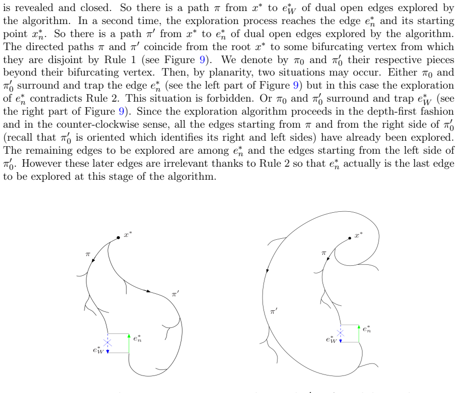
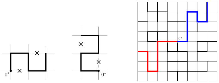
The load-bearing mechanism is an exploration algorithm for the dual forward set that reveals directed dual edges depth-first and counter-clockwise, subject to two rules that prevent re-visiting vertices or entering filled holes. Certain revealed edges are pivotal: the dual edge is the east side of a unit square and one of the other three sides has already been explored and found closed, which raises its open probability to roughly 2/3. The algorithm stops when a closed pivotal edge is found, so the explored cluster splits into 'visited clusters' separated by pivotal edges. Each visited cluster is stochastically dominated by the cluster of the origin in i.i.d. bond percolation at parameter 1/2−ε/4 under the constraint that paths never use a forbidden 'left-winding' pattern. An enhancement argument (Theorem 6.1) then shows that the forbidden-pattern restriction pushes the effective threshold above 1/2, giving exponential decay of visited clusters even at ε=0.

What would settle it

Search the finite configuration space of the 6×5 box In(Be): for each configuration outside the box, check whether the inclusion PivOut_Be ∩ RTe ⊂ {Q(e) is pivotal} holds for the map Te of Lemma 6.7. A single configuration where a good p-edge is pivotal but no deterministic local change inside the box makes Q(e) pivotal would disprove inequality (17); equivalently, compute the probability that a pivotal p-edge's associated q-edge cannot be made pivotal and show it exceeds zero for some n and e.

Watch

Extended reading notes

Core claim

On the paper's own terms, the central discovery is Theorem 2.3: pc(2)<1/2, and consequently the 2-neighbor graph percolates on $Z^{2}$. To reach it the authors work in the (2,ε)-model, where each vertex has exactly two outgoing edges plus a third with probability ε, so every directed edge is open with probability 1/2+ε/4. They prove that the dual forward set of the origin has subexponential tail decay (Theorem 3.1), and at ε=0 this requires showing that i.i.d. bond percolation with a forbidden local pattern has threshold strictly above 1/2 (Theorem 6.1). The argument also yields as corollaries that the d-neighbor graph percolates in Z^d for all d≥2 and that the directed-corner model has critical parameter below 1/2.

Load-bearing premise

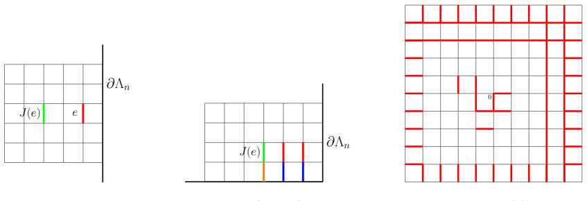
The argument hinges on the claim that inside every 6×5 box around a pivotal edge one can always locally rewrite the configuration so that a q-edge becomes pivotal while no new forbidden pattern is created; if even one boundary or origin-position subcase admits no such local rewrite, the enhancement comparison and hence the strictly-below-1/2 percolation conclusion would fail.

Editorial extensions

If this is right

The planar 2-neighbor graph percolates, so a fixed out-degree of two is enough for an infinite directed open path in Z^2.
The critical parameter satisfies 0.373 < pc(2) < 0.5, refining the earlier known lower bound with the connective constant bound of [PT00].
For every d≥2, the d-neighbor graph percolates in Z^d (Corollary 2.4).
The directed-corner model also percolates for some p<1/2 (Theorem 2.8).
At equal mean degree two, the degree-constrained model percolates while i.i.d. directed bond percolation does not: pc < piid_c = 1/2 < paon_c (Corollary 2.9).

Reading between the lines

Editorial extensions of the paper, not claims the author makes directly.

If the local-surgery comparison is uniform, the forbidden-pattern threshold is separated from 1/2 by a positive amount, so any planar directed model whose exploration process forbids the same left-winding pattern should percolate below 1/2; the ρ-family of isotropic degree-two models interpolating between the north-south-east-west and directed-corner models is a natural testbed.
The enhancement proof gives a finite certificate: each of the finitely many boundary and origin-position subcases in Lemmas 6.7 and 6.9 could in principle be checked by exhaustive enumeration of 6×5 boxes, which would convert the sketch into a verified inequality and possibly yield an explicit ε′.
A concrete prediction beyond the paper is that the percolation probability at p=1/2 decreases as the model interpolates from opposite-edge pairs to corner pairs, matching the conjecture that lower geometric variability favours percolation; computer simulations on the same exploration process could test this ordering before a rigorous proof is found.

Share X Bluesky LinkedIn Reddit HN

Editorial analysis

A structured set of objections, weighed in public.

Desk editor's note, referee report, and a circularity audit.

Desk Editor's Note

read the letter

The main theorem is real and the high-level argument holds up. The planar 2-neighbor graph percolates, and pc(2) < 1/2. This was conjectured in [JKLT23] and had been open. The proof is not a repackaging; the exploration algorithm, the pivotal-edge decomposition, and especially the non-essential enhancement argument for forbidden-pattern percolation are genuinely new. The byproduct result—that i.i.d. bond percolation with those forbidden local patterns has threshold strictly above 1/2—is also interesting.

The paper is careful about the critical case ε = 0, which is exactly where the enhancement comes in, and it handles that case in a self-contained section. The block renormalization step is standard and clean.

The soft spot is Section 6. Lemmas 6.7 and 6.9 build local modification maps Te and Se that are supposed to convert any pivotal p-edge into a pivotal q-edge by changing edges in a 6x5 box. The text gestures at the construction, refers to an external website for “all possible cases,” and in Lemma 6.9 explicitly leaves details to the reader. These maps are load-bearing: a single bad subcase would break the derivative comparison (Proposition 6.3), hence Theorem 6.1, hence the exponential decay for ε = 0. That is a genuine verification gap, not a cosmetic omission.

How much does it matter? I do not think it signals a wrong proof. The construction is explicit, the figures help, and the surrounding argument is coherent. It reads like a paper where the authors got the main theorem right and under-documented the hardest local case check. A diligent referee could either work through the cases or require the authors to expand the appendix. No code or formalization is provided, which would have helped, but that is not standard for this subfield.

The rest of the paper—domination by constrained bond percolation, the subgeometric number of pivotal edges, the duality setup—is well supported. The citation pattern is appropriate, building on [JKLT23], [AG91], [BBR14], and [Gri99] without overclaiming.

Verdict: this deserves a serious referee. I would send it to peer review with the clear instruction that Section 6 must be made self-contained or the missing case checks supplied. The result is significant enough that the case-checking burden is worth it. I would cite it if I worked on directed percolation or degenerate random environments, and I would likely bring it to reading group to discuss the enhancement technique.

Referee Report

3 major / 5 minor

Summary. The paper proves that the planar 2-neighbor directed graph percolates, i.e., pc(2) < 1/2, resolving a conjecture from [JKLT23]. The proof combines a duality and exploration algorithm for the dual forward set, a decomposition of the explored cluster into visited clusters separated by pivotal edges, a domination of each visited cluster by constrained i.i.d. bond percolation, and a block renormalization step. The critical ε = 0 case requires an enhancement argument (Section 6) showing that the forbidden-pattern constraint strictly increases the percolation threshold above 1/2. A secondary result establishes pcorn_c < 1/2 for the directed-corner model.

Significance. If correct, this settles a natural open problem and provides a rigorous example where a fixed-degree constraint is beneficial for percolation compared to i.i.d. directed percolation at the same expected degree. The enhancement argument for non-essential enhancements with forbidden patterns is of independent interest, as is the byproduct that bond percolation with forbidden local patterns has threshold strictly above 1/2. The high-level structure is coherent, the argument is parameter-free, and the proof invokes standard results (planar duality, the 1/2 critical threshold, and the LSS97 domination theorem) appropriately. However, the manuscript's load-bearing local modifications in Section 6 are not fully proved in the text, with a companion website and 'left to the reader' invoked for essential cases. No machine-checked proofs or reproducible code are provided, so the current version is not yet complete.

major comments (3)

[§6.3.1 (Lemma 6.7)] The construction of the map Te, used to prove inequality (17), is not fully specified. The printed proof gives a semi-explicit construction but explicitly refers to an external website for 'a concrete visualization of the construction in all possible cases' and treats several subcases (o inside Be, Be intersecting ∂Λn, x′ = y′, and the choice of entry/exit pairs) only heuristically. Item (iii) of the lemma is load-bearing: it must hold for every entry/exit pair and every boundary/position subcase, and a single failure would invalidate (17), hence Proposition 6.3, Theorem 6.1, and the ε = 0 case of Theorem 3.1. The companion website is not a substitute for a rigorous proof, and no machine-checked verification is supplied.
[§6.3.2 (Lemma 6.9)] The map Se for bad edges is only sketched. For categories (a)–(e), the proof states 'We leave the details to the reader', and for category (f) it again leaves the three subcases to the reader with only a schematic figure. Since inequality (18) — and hence the bound on the total contribution of bad edges in Lemma 6.6 — depends entirely on this lemma, the proof of Proposition 6.3 is incomplete at this point. As with Lemma 6.7, this gap is not cosmetic because the local modification must work in all boundary and origin-position cases.
[§7 (Lemma 7.1)] The exponential tail estimate for the number of pivotal edges in the directed-corner model also defers 'the verification of the intermediate cases to the reader'. While Theorem 2.8 is a byproduct rather than the main theorem, the same standard of completeness should apply, and the omitted cases are not trivial given the auto-open pivotal-edge analysis in the proof.

minor comments (5)

[§5.2, Step 1, inequality (10)] The text says 'All these probabilities are smaller than qε', but in the first case the probability equals qε = 1/2 − ε/4; it should say 'at most qε'.
[§6.3.1, proof of inequality (17)] The proof claims that In(Be) contains 71 p-edges, but the box B is defined as the 6×5 rectangle minus its four corners, which gives 63 p-edges with both endpoints in B. The bound with exponent 71 remains valid because p(1−p) ≤ 1/4, but the stated count is incorrect and should be corrected or replaced by 'at most 71'.
[§6.3, definition of Ibad] The displayed set Ibad lists eight edges, but the entry {(−1,−1),(−1,0)} appears twice; this appears to be a typographical repetition that should be cleaned up.
[§4.2, pivotal probability computation] The display computing the conditional probability of a pivotal edge being open is garbled in the text; the final value (2/3)(1−ε/4)/(1+ε/2) is clear, but the intermediate notation should be typeset cleanly.
[§3.2, Lemma 3.2 proof] The notation 'z_i^* := (i+1/2, −1/2)' is used for dual start points; later in the proof the union bound is written as 3L × Ce^{-cL^{1/4}}, which is correct, but the phrase 'for some integer 0 ≤ i ≤ 3L−1' should specify that i is an index over the left side of the rectangle, since the dual path starts on that side.

Circularity Check

0 steps flagged · score 0.0 of 10

No significant circularity: the main derivation is self-contained and does not reduce to fitted parameters, definitions, or load-bearing self-citations.

full rationale

The paper's central claim, pc(2) < 1/2, is derived from the model definition through an independent chain: duality, an exploration algorithm, a decomposition into visited clusters separated by pivotal edges, domination by i.i.d. bond percolation with a forbidden pattern, and an enhancement argument for that constrained percolation model. No fitted parameter is introduced and then renamed as a prediction; the threshold inequality is proved by comparing pivotal probabilities via explicit local modifications. The only self-citation to prior work by the same authors is [JKLT23], used to state the conjecture and to derive Corollary 2.4 in all dimensions from the d = 2 result; it is not load-bearing for Theorem 2.3 itself. The paper does contain explicitly deferred verification, notably Lemma 6.9 ('We leave the details to the reader') and part of Lemma 7.1 ('We leave the verification of the intermediate cases to the reader'), and it refers to a companion website for case-by-case visualizations. These are completeness or correctness gaps, not circularity: they do not make the conclusion an input to the proof. The enhancement comparison in Theorem 6.1 is an independent statement about Bernoulli bond percolation with forbidden patterns, proved from Russo's formula and local coupling inequalities, not from the percolation claim being established.

Assumptions & free parameters 0 free parameters · 4 assumptions · 1 invented entities

All constants in the proof are existential or computed from standard bounds; none are fitted to simulations. The model definition is the only input. Axioms are standard planar percolation facts, the LSS97 domination theorem, and the rigidity property of the model (at least two outgoing edges per vertex). The diagonal q-edges are an auxiliary proof device, not a physical claim.

assumptions (4)

standard math Planar crossing duality: no open primal crossing in a rectangle implies an open dual crossing.
Invoked in the proof of Lemma 3.2 to translate non-percolation of primal rectangles into large dual forward sets.
standard math Bernoulli bond percolation on Z^2 has critical point 1/2 and subcritical exponential decay of connection probabilities.
Used in Lemma 2.5 and in Sections 5 and 6 to compare the constrained model to subcritical percolation; cited to [Gri99].
standard math Liggett-Schonmann-Stacey domination by product measures for m-dependent fields.
Used in Section 3.2 to convert lower bounds on block marginals into percolation of the block field; cited to [LSS97].
domain assumption Every primal vertex has at least two outgoing edges, so a dual exploration path cannot contain a left winding around a single primal vertex.
A direct consequence of the model definition, used in the proof of inclusion (14) in Section 5.2 to restrict undirected paths to forbidden-pattern-free routes.

invented entities (1)

Diagonal q-edges in the enhanced bond percolation model
purpose: Auxiliary edges introduced to prove Theorem 6.1 by enhancement; they are not part of the original 2-neighbor graph.
The q-edges are a proof device used to bypass forbidden patterns in the enhanced model. They carry no physical claim and no external falsifiable prediction.

how reviews work

0 comments

Cite this review

Pith. "Pith review of The Planar Lattice Two-Neighbor Graph Percolates." pith.science (2026). https://pith.science/paper/AOHAQLAI

@misc{pith2026241220781,
  author       = {Pith},
  title        = {Pith review of: The Planar Lattice Two-Neighbor Graph Percolates},
  year         = {2026},
  howpublished = {\url{https://pith.science/paper/AOHAQLAI}},
  note         = {Machine review of arXiv:2412.20781}
}

read the original abstract

The k-neighbor graph is a directed percolation model on the hypercubic lattice Z d in which each vertex independently picks exactly k of its 2d nearest neighbors at random, and we open directed edges towards those. We prove that the 2-neighbor graph percolates on Z 2 , i.e., that the origin is connected to infinity with positive probability. The proof rests on duality, an exploration algorithm, a comparison to i.i.d. bond percolation under constraints as well as enhancement arguments. As a byproduct, we show that i.i.d. bond percolation with forbidden local patterns has a strictly larger percolation threshold than 1/2. Additionally, our main result provides further evidence that, in low dimensions, less variability is beneficial for percolation.

Figures

Figures reproduced from arXiv: 2412.20781 by the authors.

**Figure 1.** (a) A possible local configuration of the planar 2-neighbor model and (b) the resulting forward cluster of the origin. Note that, since the model is directed, the relation x ⇝ y is not reflexive. The original motivation for studying the k-neighbor graph on Z d comes from a continuum percolation model initially introduced in [HM96]. In that work, the authors consider an homogeneous Poisson point process on R d (say … view at source ↗

**Figure 2.** (a) A possible local configuration of the northsouth-eastwest model with p = 1/2 and (b) the resulting forward cluster of the origin. Theorem 2.8 (Upper bound for the directed-corner model). It holds that p corn c < 1/2. (a) (0,0) (b) (0,0) [PITH_FULL_IMAGE:figures/full_fig_p006_2.png] view at source ↗

**Figure 3.** (a) A possible local configuration of the directed corner model with p = 1/2 and (b) the resulting forward cluster of the origin. 2.3.4. Comparison. From our rigorous analysis we can formulate the following comparison of critical values. Corollary 2.9 (Comparison). For d = 2, we have that pc < piid c = 1/2 < paon c . Additionally, our simulations suggest the following strict order of percolation thresholds in two sp… view at source ↗

Figures from the paper (25 more)

**Figure 4.** Figure 4: Primal edge in red and its dual edge in blue. This color code will be conserved for the whole paper. As primal edges, dual edges are also directed. Given a configuration ω ∈ Ω, we define its dual configuration ω ∗ as the element of Ω ∗ = {0, 1} E ∗ such that ∀e ∈ E, ω∗…

**Figure 5.** Figure 5: Two neighboring blocks, centered at Lz and Lz′ with z ′ = z + (1, 0), and the corresponding open cycles realizing the events G(Lz, 3L) and G(Lz′ , 3L). Theorem 3.1 allows us to establish the next result whose proof is postponed to the end of the section. Lemma 3.2. The…

**Figure 6.** Figure 6: Left: A representation of the event Cross(L). Right: Considering four rotated and shifted copies of the event Cross(L) and glueing the corresponding open paths γi , i = 1, 2, 3, 4, we obtain a cycle surrounding the origin o in B(o, 3L/2)\B(o, L/2). The event G(o, 3L) …

**Figure 7.** Figure 7: In the exploration algorithm, edges are explored in the counterclockwise sense. In addition, our exploration algorithm will respect two limiting rules detailed below. Let Vn ⊂ (Z 2 ) ∗ be the set of vertices already explored (or visited) by the exploration process unt…

**Figure 8.** Figure 8: The directed dual edge e ∗ n is the east edge of the unit square and is represented in green. It is pivotal for the exploration process since the west (dual) edge e ∗ W has been already visited by the exploration process and is closed (in light blue). This is why its p…

**Figure 9.** Figure 9: Both pictures represent two paths π and π ′ performed during the exploration process of the forward set of x ∗ until the n-th step of the algorithm. π and π ′ respectively reach the directed dual edges e ∗ W and e ∗ n : e ∗ W has been previously revealed and is closed …

**Figure 10.** Figure 10: Unlike [PITH_FULL_IMAGE:figures/full_fig_p016_10.png]

**Figure 11.** Figure 11: Schematic representation of the structure of the explored forward cluster ExFor(x ∗ ) as the union of the k-th explored clusters (shaded) linked by pivotal edges (orange). 4.4. Proof of Theorem 3.1. In order to conclude the proof of Theorem 3.1, we need two more ingre…

**Figure 12.** Figure 12: Left: the first and second forbidden patterns. The small black crosses emphasize the fact that the corresponding edges are closed. Right: here is a configuration of the box o ∗ + Λ4 satisfying the event {o ∗ ⇝ o ∗ + ∂Λ4 without } thanks to the red path (for instance),…

**Figure 13.** Figure 13: Left: The set of revealed directed edges during the exploration process of For(x ∗ ) (associated to the dual configuration ω ∗ ). The open and closed revealed edges are respectively represented by bold and dashed arrows. In this basic example, there are no pivotal edg…

**Figure 14.** Figure 14: Left: Two diagonal edges (or q-edges) incident to the vertex (a, b). Right: A forbidden pattern and its associated diagonal edge (in green). Let us now define the family of probability measures on Ω + that we want to study. There are two layers of randomness. First, e…

**Figure 15.** Figure 15: The opening of a closed edge in the left pattern makes useless the corresponding diagonal edge. However, a new admissible open path of p-edges (i.e. without using a forbidden pattern) appears in the right pattern. We are now ready to show Russo-type formula for partia…

**Figure 16.** Figure 16: Two p-edges (in red) and their associated q-edges (in green). Indeed, some p-edges satisfy P +(e is pivotal) > 0 while P +(Q(e) is pivotal) = 0. In that case, our strategy fails. Such pathological p-edges e ∈ Ein n are of two types: • When Q(e) ∈ D/ in n (i.e., the as…

**Figure 17.** Figure 17: The vertical edge e := {(a, b),(a, b + 1)} (in red) and the box Be whose border is delimited by a black line. Moreover, the orange dots represent the points to avoid (if it is possible) according to rule (∗). See below. Note that, although e is a good p-edge, the box …

**Figure 18.** Figure 18: For good edges e and their associated forbidden pattern we only need to change the status of edges in the shaded region Be around e. If e is a pivotal p-edge, then there is at least one admissible path from the origin to the boundary of Be and at least one path connec…

**Figure 19.** Figure 19: Construction of Te(ω) when x ′ ̸= y ′ (in orange) and they are on the green path. Vertices x and y are represented by red dots. Edges {x, x′} and {y, y′} are in yellow. Blue edges are {u,(a, b)}, {(a + 2, b + 1), v} and those corresponding to the forbidden pattern ass…

**Figure 20.** Figure 20: Opening the yellow edge {x, x′} may create a forbidden pattern with the exterior of Be (represented by the dotted blue edges). However, if so, it contradicts constraint (∗) as the green vertex could have been chosen as entry/exit point. Let us first consider the case …

**Figure 21.** Figure 21: Construction of Te(ω) when x ′ ̸= y ′ (in orange) and x ′ belongs to the green path, y ′ belongs to the magenta path. To the right: we build a multicolor path π with the yellow edges {x, x′} and {y, y′}, the green edges between x ′ and u, the magenta edges between y ′…

**Figure 22.** Figure 22: Construction of Te(ω) in the case x ′ = y ′ . Next, let us study the case where Be ∩ ∂Λn ̸= ∅. The box Be exceeds Λn \∂Λn but not too much since e is a good p-edge: Be has actually to be included in Λn+1, so in particular parts of the cycle C are contained in ∂Λn. Sin…

**Figure 23.** Figure 23: Left: the bad edge e (in red) corresponding to the category (c) and the good edge J(e) (in green). Center: five bad edges are represented having the same image by the map J (in green); the red bad edges correspond to the category (c), the blue ones to the category (e)…

**Figure 24.** Figure 24: In the case where the edge e (blue) is bad because it is too close to the boundary ∂Λn, we map it to a good edge J(e) (pink) which is slightly further inside of Λn but still such that e ∈ BJ(e) . If e is pivotal for a configuration ω, then there must be at least one a…

**Figure 25.** Figure 25: (a) In the case where the edge e (black) is bad because the associated pattern contains the origin o in its interior, we map it to a good edge J(e) (pink) nearby such that this is not the case. If e is pivotal for a configuration ω, then there must be at least one ad…

**Figure 26.** Figure 26: The four different configurations of outgoing edges a vertex can choose in the directed corner model with parameter p = 1/2. The proof follows step by step the one of Theorem 2.3 and the only major difference arises when one wants to get good probabilistic bounds for …

**Figure 27.** Figure 27: Dual vertices visited by the exploration process are blue points. Open and revealed edges are depicted with blue lines while closed and revealed edges are depicted with blue dotted lines. By red lines, we indicate the primal vertices at which the states of dual edges …

**Figure 28.** Figure 28: The color code is the same as in [PITH_FULL_IMAGE:figures/full_fig_p042_28.png]

Discussion (0). Continue with ORCID to comment.

Forward citations

Cited by 1 Pith paper

Reviewed papers in the Pith corpus that reference this work. Sorted by Pith novelty score. Full citation record

Strongly-connected percolation on directed lattices
cond-mat.stat-mech 2026-07 accept novelty 6.0 of 10

Bond percolation of strongly-connected clusters on directed square lattices is in one new 2D universality class, distinct from ordinary percolation, across Manhattan, L, ice, and random-diode orientations.

Reference graph

Works this paper leans on

35 extracted references · 34 canonical work pages · cited by 1 Pith paper

[1]

Aizenman and G

M. Aizenman and G. Grimmett, Strict monotonicity for critical points in percolation and ferromagnetic models, J. Stat. Phys. 63 (1991), 817--835

work page 1991
[2]

Balister and B

P. Balister and B. Bollob \'a s, Percolation in the k -nearest neighbor graph, Recent results in designs and graphs: A tribute to Lucia Gionfriddo, Quaderni di Matematica 28 (2013), 83--100

work page 2013
[3]

Balister, B

P. Balister, B. Bollob \'a s, and O. Riordan, Essential enhancements revisited, arXiv preprint arXiv:1402.0834 (2014)

arXiv 2014
[4]

Beekenkamp, Sharpness of the phase transition for the orthant model, Math

Th. Beekenkamp, Sharpness of the phase transition for the orthant model, Math. Phys. Anal. Geom. 24 (2021), no. 4, 36

work page 2021
[5]

Chemical distance for the half-orthant model

N. Beaton, M. Holmes, and X. Huang, Chemical distance for the half-orthant model, arXiv preprint arXiv:2401.03647 (2024)

work page Pith review arXiv 2024
[6]

Bollob \'a s and O

B. Bollob \'a s and O. Riordan, Percolation, Cambridge University Press, 2006

work page 2006
[7]

de Lima, S

B. de Lima, S. Martineau, H. Sanna, and D. Valesin, Approximation on slabs and uniqueness for B ernoulli percolation with a sublattice of defects , ALEA Lat. Am. J. Probab. Math. Stat. 19 (2022), no. 2, 1767--1797

work page 2022
[8]

de Lima, R

B. de Lima, R. Sanchis, D. dos Santos, V. Sidoravicius, and R. Teodoro, The constrained-degree percolation model, Stoch. Process. Their Appl. 130 (2020), no. 9, 5492--5509

work page 2020

Show all 35 references

[9]

Friedli, D

S. Friedli, D. Ioffe, and Y. Velenik, Subcritical percolation with a line of defects, Ann. Probab. 41 (2013), no. 3B, 2013 -- 2046

2013
[10]

Grimmett and S

G. Grimmett and S. Janson, Random graphs with forbidden vertex degrees, Random Struct. Algorithms. 37 (2010), no. 2, 137--175

2010
[11]

Grimmett and Z

G. Grimmett and Z. Li, The 1-2 model, Contemp. Math 969 (2017), 139--152

2017
[12]

Gou \'e r \'e and R

J.-B. Gou \'e r \'e and R. Marchand, Nonoptimality of constant radii in high dimensional continuum percolation, Ann. Appl. Probab. 44 (2016), no. 1, 307--323

2016
[13]

Gou \'e r \'e , Percolation in a multiscale B oolean model , ALEA Lat

J.-B. Gou \'e r \'e , Percolation in a multiscale B oolean model , ALEA Lat. Am. J. Probab. Math. Stat. (2014), 11--1

2014
[14]

Ghosh and Y

S. Ghosh and Y. Peres, Rigidity and tolerance in point processes: Gaussian zeros and Ginibre eigenvalues , Duke Math. J. 166 (2017), no. 10, 1789--1858

2017
[15]

Grimmett, Percolation, Springer, 1999

G. Grimmett, Percolation, Springer, 1999

1999
[16]

Algorithms

, Infinite paths in randomly oriented lattices, Random Struct. Algorithms. 18 (2001), no. 3, 257--266

2001
[17]

333, Springer, 2006

, The random-cluster model, vol. 333, Springer, 2006

2006
[18]

Holroyd and Z

A. Holroyd and Z. Li, Constrained percolation in two dimensions, Ann. Inst. Henri Poincar \'e D 8 (2021), no. 3, 323--375

2021
[19]

a ggstr \

O. H \"a ggstr \"o m and R. Meester, Nearest neighbor and hard sphere models in continuum percolation, Random Struct. Algorithms 9 (1996), no. 3, 295--315

1996
[20]

Holroyd and T

A. Holroyd and T. Soo, Insertion and deletion tolerance of point processes, Electron. J. Probab. 18 (2013), 24, Id/No 74

2013
[21]

Holmes and Th

M. Holmes and Th. Salisbury, Degenerate random environments, Random Struct. Algorithms. 45 (2014), no. 1, 111--137

2014
[22]

, Phase transitions for degenerate random environments, ALEA Lat. Am. J. Probab. Math. Stat. 18 (2021), 707 -- 725

2021
[23]

, A shape theorem for the orthant model, J. Stat. Phys. 49 (2021), no. 3, 1237 -- 1256

2021
[24]

Iliev, E

G. Iliev, E. Janse van Rensburg, and N. Madras, Phase diagram of inhomogeneous percolation with a defect plane, J. Stat. Phys. 158 (2015), 255--299

2015
[25]

Jacobsen, Critical points of P otts and O(N) models from eigenvalue identities in periodic temperley--lieb algebras , J

J. Jacobsen, Critical points of P otts and O(N) models from eigenvalue identities in periodic temperley--lieb algebras , J. Phys. A: Math. Theor. 48 (2015), no. 45, 454003

2015
[26]

Jahnel, J

B. Jahnel, J. K \"o ppl, B. Lodewijks, and A. T \'o bi \'a s, Percolation in lattice k -neighbor graphs, arXiv preprint arXiv:2306.14888 (2023)

2023 arXiv
[27]

Kenyon, A

R. Kenyon, A. Okounkov, and S. Sheffield, Dimers and amoebae, Ann. Math. (2006), 1019--1056

2006
[28]

1, 71--95

Thomas M Liggett, Roberto H Schonmann, and Alan M Stacey, Domination by product measures, The Annals of Probability 25 (1997), no. 1, 71--95

1997
[29]

Newman and C

Ch. Newman and C. Wu, Percolation and contact processes with low-dimensional inhomogeneity, Ann. Probab. 25 (1997), no. 4, 1832--1845

1997
[30]

Peres and A

Y. Peres and A. Sly, Rigidity and tolerance for perturbed lattices, arXiv preprint arXiv:1409.4490 (2014)

2014 arXiv
[31]

P \"o nitz and P

A. P \"o nitz and P. Tittmann, Improved upper bounds for self-avoiding walks in Z ^d , Electron. J. Comb. 7 (2000), R21--R21

2000
[32]

Quintanilla and R

J. Quintanilla and R. Ziff, Asymmetry in the percolation thresholds of fully penetrable disks with two different radii, Phys. Rev. E: Stat. Nonlin. Soft Matter Phys. 76 (2007), no. 5, 051115

2007
[33]

van den Berg and A

J. van den Berg and A. Ermakov, A new lower bound for the critical probability of site percolation on the square lattice, Random Struct. Algorithms. 8 (1996), no. 3, 199--212

1996
[34]

Wierman, AB percolation: a brief survey , Banach Cent

J. Wierman, AB percolation: a brief survey , Banach Cent. Publ. 25 (1989), no. 1, 241--251

1989
[35]

Zhang, A note on inhomogeneous percolation, Ann

Y. Zhang, A note on inhomogeneous percolation, Ann. Probab. (1994), 803--819

1994

Pith tools

Reviewed August 10, 2026 · model on record in the stance chip above.

[1] [1]

Aizenman and G

M. Aizenman and G. Grimmett, Strict monotonicity for critical points in percolation and ferromagnetic models, J. Stat. Phys. 63 (1991), 817--835

work page 1991

[2] [2]

Balister and B

P. Balister and B. Bollob \'a s, Percolation in the k -nearest neighbor graph, Recent results in designs and graphs: A tribute to Lucia Gionfriddo, Quaderni di Matematica 28 (2013), 83--100

work page 2013

[3] [3]

Balister, B

P. Balister, B. Bollob \'a s, and O. Riordan, Essential enhancements revisited, arXiv preprint arXiv:1402.0834 (2014)

arXiv 2014

[4] [4]

Beekenkamp, Sharpness of the phase transition for the orthant model, Math

Th. Beekenkamp, Sharpness of the phase transition for the orthant model, Math. Phys. Anal. Geom. 24 (2021), no. 4, 36

work page 2021

[5] [5]

Chemical distance for the half-orthant model

N. Beaton, M. Holmes, and X. Huang, Chemical distance for the half-orthant model, arXiv preprint arXiv:2401.03647 (2024)

work page Pith review arXiv 2024

[6] [6]

Bollob \'a s and O

B. Bollob \'a s and O. Riordan, Percolation, Cambridge University Press, 2006

work page 2006

[7] [7]

de Lima, S

B. de Lima, S. Martineau, H. Sanna, and D. Valesin, Approximation on slabs and uniqueness for B ernoulli percolation with a sublattice of defects , ALEA Lat. Am. J. Probab. Math. Stat. 19 (2022), no. 2, 1767--1797

work page 2022

[8] [8]

de Lima, R

B. de Lima, R. Sanchis, D. dos Santos, V. Sidoravicius, and R. Teodoro, The constrained-degree percolation model, Stoch. Process. Their Appl. 130 (2020), no. 9, 5492--5509

work page 2020