REVIEW 3 major objections 3 minor 40 references
Analysis of Two-Dimensional Feedback Systems over Networks Using Dissipativity
T0 review · 3 major / 3 minor · reviewed 2026-08-14 · deepseek-v4-flash
Pith's one-line read 2-D feedback systems can stay L2-stable over digital networks
desk verdict A new 2-D dissipativity extension with real ideas, but Theorem 1's 'exact' sampling is not exact, and the example leans on it. read the letter →
The pith
A machine-rendered reading of the paper's core claim, the machinery that carries it, and where it could break.
The reading
What carries the argument
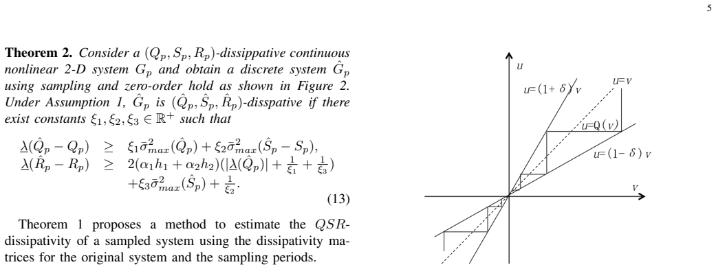
The argument is carried by a 2-D version of QSR-dissipativity with a separable storage function $V(x_h,x_v)=V_h(x_h)+V_v(x_v)$, and by the reduced passivity indices called IF-OFP levels $(\rho,\nu)$. Sampling is handled through a bound on the sampling error $\Delta y_p$ in terms of the sampling periods $h_1,h_2$ and gain constants $\alpha_1,\alpha_2$; logarithmic quantization is handled through the sector bound $|\Delta v|\le \delta|v|$; and the event-triggering scheme compares the accumulated output error against a threshold derived from the same passivity levels, so that the combined supply rate remains negative definite.
What would settle it
A single numerical counterexample—a plant-controller pair satisfying the passivity inequalities of Theorem 3 and the conditions of Theorem 4 whose sampled, quantized, event-triggered closed-loop output diverges—would refute the central claim; the Section IV heat-exchanger example with $h_1=h_2=0.1$, $\delta_p=\delta_c=0.04$, $K=3$, and $N_1=40$ is the concrete configuration to test.
Extended reading notes
Core claim
The paper's central claim is that the $\mathcal{L}_2$ stability of a 2-D feedback interconnection is preserved under the main effects of a digital link—sampling, logarithmic quantization, and event-triggered transmission—provided explicit dissipativity inequalities hold. For quantization, the closed-loop map is $\mathcal{L}_2$-stable whenever the passivity surplus of each subsystem dominates the degradation introduced by the quantizer, as expressed by the two inequalities $\rho_p + \nu_c > (\delta_p^2+2\delta_p)|\nu_c| + (1+\beta_2^2)\delta_p^2 + \frac{1}{2\beta_1}$ and its mirror image. For event-triggered communication, the paper shows that triggering at times selected by condition (22) yields finite $\mathcal{L}_2$-gain on a bounded spatial domain, so transmissions can be reduced without destroying stability.
Load-bearing premise
The load-bearing premise is Assumption 2, which restricts the event-triggered result to 2-D systems with one coordinate on a bounded spatial domain: Theorem 4 proves finite $\mathcal{L}_2$-gain only for that case, and the extension to infinite spatial domains is a sketched remark rather than a theorem.
Editorial extensions
If this is right
- If Theorem 3 is right, a designer can guarantee $\mathcal{L}_2$ stability by tuning the quantizer densities and the auxiliary constants $\beta_1,\beta_2$, using only the plant and controller IF-OFP levels.
- If Theorem 4 is right, event-triggered 2-D control can reduce transmissions along the vertical coordinate while preserving a finite $\mathcal{L}_2$-gain on bounded spatial domains.
- If Theorems 1 and 2 are right, sampling periods $h_1,h_2$ can be chosen from the LMI or from the inequalities to keep the sampled system dissipative.
- Lemma 2 extends the classical small-gain style passivity theorem to 2-D IF-OFP systems, giving a simple sufficient condition $\nu_2+\rho_1>0$ and $\nu_1+\rho_2>0$ for feedback stability.
Reading between the lines
- The paper's Remark 4 suggests the bounded-spatial-domain assumption can be relaxed by gridding the domain and applying the same trigger rule on each interval; if that extension holds, the method would apply to long spatial extents such as pipelines or convection processes, but the extension is not proved as a theorem.
- The separable storage function $V_h+V_v$ is intentionally conservative; using less conservative 2-D Lyapunov functions could sharpen the passivity degradation bounds and allow less restrictive triggering thresholds.
- The explicit dependence of the stability conditions on $\delta_p,\delta_c$ suggests a co-design problem: communication rate (quantizer density) and event-trigger thresholds can be traded directly against controller passivity levels.
- The framework treats the plant and controller asymmetrically only through their passivity levels and quantizer densities, so the same conditions could be adapted to other 2-D architectures such as iterative learning control or distributed spatial systems.
Signed reviews
Editorial analysis
A structured set of objections, weighed in public.
Referee Report
Summary. The paper develops a dissipativity-based framework for analyzing L2 stability of two-dimensional (2-D) feedback systems interconnected over a digital network. It introduces QSR-dissipativity definitions for continuous and discrete 2-D Roesser systems, then treats three network-induced effects sequentially: sampling with zero-order hold, logarithmic quantization, and event-triggered transmission. For linear sampled 2-D systems it provides an LMI condition (Theorem 1); for nonlinear systems it gives a sampling-error bound and a dissipativity degradation condition (Lemma 3 and Theorem 2). It then analyzes how logarithmic quantization degrades IF-OFP passivity levels (Theorem 3) and proposes an event-triggering rule that preserves a finite L2-gain on bounded spatial domains (Theorem 4). A hyperbolic PDE example is used to illustrate the conditions and the closed-loop behavior.
Significance. The topic is timely: networked control of 2-D systems is relatively unexplored, and the modular decomposition into sampling, quantization, and event-triggering is a sensible program. The quantization analysis in Theorem 3 and the event-triggering scheme, once its typographical inconsistencies are fixed, provide explicit and verifiable sufficient conditions, and the running PDE example is instructive. I credit the authors for stating the bounded-domain assumption explicitly in Assumption 2 and for making the triggering rule implementable as an online check of condition (22). However, the two sampling results at the foundation of the paper are not established as stated: Theorem 1's discrete model is an approximation rather than the exact sampled model, and the proof of Theorem 2 uses an inequality that fails for negative-definite Qp_hat. Because the example's passivity levels are computed from Theorem 1, the numerical validation does not currently back the advertised guarantees. The contribution can be salvaged, but the manuscript needs substantive correction.
major comments (3)
- [Section III-A, Theorem 1; Appendix D, Eq. (8)] The discrete model in (8) is not the exact sampled model of the continuous Roesser system (2). In the singular case covered by Remark 1, take A11=A22=0, A12=A21=1, B=0. With boundary data xh(0,z2)=e^{z2} and xv(z1,0)=e^{z1}, the exact solution is xh(z1,z2)=xv(z1,z2)=e^{z1+z2}, so xh(h1,0)=e^{h1}; the recurrence (8) gives xh(h1,0)=1+h1. These differ for h1>0. Therefore the LMI (7) certifies QSR-dissipativity of a different, approximate discrete system rather than of the actual sampled plant, and the IF-OFP levels computed in Section IV from this model do not by themselves certify stability of the true sampled feedback loop. This point needs to be fixed by deriving an exact sampled model, or by explicitly treating the discretization as an approximation with a separate error analysis.
- [Section III-A, Theorem 2 and Appendix C] The proof's inequality Δy_p^T Qp_hat Δy_p ≥ |λ_min(Qp_hat)| |Δy_p|^2 is valid only when Qp_hat is positive semidefinite. For example, if Qp_hat = -I, the left side is -|Δy_p|^2, which is not bounded below by |λ_min(Qp_hat)| |Δy_p|^2 = |Δy_p|^2. Since Theorem 2 does not require Qp_hat ⪰ 0 and condition (13) uses the absolute value, the theorem as stated is not proved. In addition, the second inequality in (13) writes 2(α1 h1 + α2 h2), while the proof in Appendix C uses Lemma 3's 2(α1^2 h1^2 + α2^2 h2^2); the statement and proof need to be reconciled, and the correct form should follow from Lemma 3.
- [Section III-C, Theorem 4 statement and proof] The displayed definition of q2 in Theorem 4 is not the same as the q2 used in the proof and in Eq. (32): the theorem statement has |ν_c| and δ_p^2 where the proof has |ν_p| and δ_c^2. This is more than a typo because the threshold in (22) depends on q1 and q2 through ϵ^2; a reader implementing the printed condition obtains a different event-triggering rule. The theorem's conclusion should also be stated as finite L2-gain on a bounded spatial domain (Definition 4), which is weaker than the global L2 stability mentioned in the abstract.
minor comments (3)
- [Abstract and Section I] The abstract and introduction state global L2 stability, but Theorem 4 only gives finite L2-gain on a bounded spatial domain (Definition 4); please add an explicit scope statement where the main results are summarized.
- [Section IV, Eq. (26)] The example writes D=∅; it should be D=0 or the corresponding zero matrix of appropriate dimensions, since the output equation y = C x + D u is otherwise underspecified.
- [Section III-A, Theorem 1] Theorem 1 assumes A11 and A22 are nonsingular 'for simplicity', but Remark 1 already extends the formulas to the singular case via series; please state in the theorem whether the nonsingularity assumption is part of the hypothesis or whether Remark 1 formally extends the statement.
Circularity Check
No significant circularity: the stability and dissipativity conditions are proved from stated assumptions rather than fitted to outcomes or imported as load-bearing self-citations.
full rationale
The derivation chain is self-contained at the level of circularity. Theorem 1 gives an LMI sufficient condition for QSR-dissipativity of a discrete model obtained from the continuous Roesser matrices; the condition is derived from the storage-function decrement and is not obtained by fitting any parameter to a targeted conclusion. Theorem 2 compares the continuous and sampled supply rates, uses Lemma 3 (proved from Assumption 1) to bound the sampling error, and then states sufficient inequalities; the dissipativity matrices Qhatp, Shatp, Rhatp appear as design variables, not as fitted outputs. Theorem 3 is a direct sector-bound calculation from IF-OFP supply rates and the logarithmic quantizer bound, giving explicit sufficient conditions; when the quantization densities vanish it reduces to Lemma 2, a standard interconnection result, not a self-citation. Theorem 4 constructs an event-triggering threshold by completing the square in the proof; the trigger condition is deliberately chosen to enforce the supply-rate inequality, so it is a synthesis condition rather than a prediction forced by the assumptions. The paper cites prior work by the same group ([19], [26], [27], [31]) for logarithmic quantization, derivative-boundedness assumptions, and componentwise quantizer operation, but these are contextual assumptions or standard tools; the load-bearing bounds and inequalities are derived in the paper from Definitions 1-3 and the stated assumptions. No fitted parameter is renamed as a prediction, and no uniqueness theorem or ansatz is imported to forbid alternatives. Remark 4 explicitly describes the infinite-domain extension as a gridding sketch rather than a theorem; that is a limitation on scope, not a circular step. Whether Theorem 1's sampled model exactly represents the continuous Roesser plant is a modeling-accuracy and correctness question, not an instance of circularity.
Assumptions & free parameters
free parameters (4)
- alpha_1, alpha_2
- xi_1, xi_2, xi_3
- beta_1, beta_2 =
beta_1=36, beta_2=56 in example
- theta_1, theta_2 =
theta_1=theta_2=0.5 in example
assumptions (6)
- domain assumption The proposed 2-D QSR-dissipativity definition with separable additive storage function V = Vh + Vv captures the relevant energy balance.
- standard math Lemma 1: QSR-dissipativity with Q < 0 implies L2 stability for 2-D systems.
- standard math Lemma 2: feedback interconnection of two IF-OFP 2-D systems is L2 stable when nu_2 + rho_1 > 0 and nu_1 + rho_2 > 0.
- domain assumption Assumption 1: the output directional derivatives are bounded in L2 by alpha_1, alpha_2 times the input norm.
- domain assumption Assumption 2: one coordinate of the 2-D system is a bounded spatial domain.
- standard math The logarithmic quantizer satisfies the sector bound |Delta v| <= delta |v|.
Cite this review
Pith. "Pith review of Analysis of Two-Dimensional Feedback Systems over Networks Using Dissipativity." pith.science (2026). https://pith.science/paper/AWWZXI5R
@misc{pith2026190801654,
  author       = {Pith},
  title        = {Pith review of: Analysis of Two-Dimensional Feedback Systems over Networks Using Dissipativity},
  year         = {2026},
  howpublished = {\url{https://pith.science/paper/AWWZXI5R}},
  note         = {Machine review of arXiv:1908.01654}
}
abstract
This paper investigates the closed-loop $\mathcal{L}_2$ stability of two-dimensional (2-D) feedback systems across a digital communication network by introducing the tool of dissipativity. First, sampling of a continuous 2-D system is considered and an analytical characterization of the $QSR$-dissipativity of the sampled system is presented. Next, the input-feedforward output-feedback passivity (IF-OFP), a simplified form of $QSR$-dissipativity, is utilized to study the framework of feedback interconnection of two 2-D systems over networks. Then, the effects of signal quantization in communication links on dissipativity degradation of the 2-D feedback quantized system is analyzed. Additionally, an event-triggered mechanism is developed for 2-D networked control systems while maintaining $\mathcal{L}_2$ stability of the closed-loop system. In the end, an illustrative example is provided.
Figures


Figures from the paper (3 more)


Reference graph
Works this paper leans on
- [1]
-
[2]
T. S. Huang, Two-Dimensional Digital Signal Processing II: Transforms and Median Filters . Secaucus, NJ, USA: Springer-Verlag New York, Inc., 1981
work page 1981
- [3]
-
[4]
A. Benzaouia, A. Hmamed, and F. Tadeo, Two-Dimensional Systems: From Introduction to State of the Art , 1st ed. Springer Publishing Company, Incorporated, 2015
work page 2015
-
[5]
Stability of two-dimensional linear systems with singularities on the stability boundary using LMIs,
S. Knorn and R. H. Middleton, “Stability of two-dimensional linear systems with singularities on the stability boundary using LMIs,” IEEE Transactions on Automatic Control, vol. 58, no. 10, pp. 2579–2590, Oct 2013
work page 2013
-
[6]
N. K. Bose, Applied Multidimensional Systems Theory, 2nd ed. Springer Publishing Company, Incorporated, 2017
work page 2017
- [7]
-
[8]
A discrete state-space model for linear image processing,
R. Roesser, “A discrete state-space model for linear image processing,” IEEE Transactions on Automatic Control , vol. 20, no. 1, pp. 1–10, Feb 1975
work page 1975
Show all 40 references
-
[9]
Doubly-indexed dynamical systems: State-space models and structural properties,
E. Fornasini and G. Marchesini, “Doubly-indexed dynamical systems: State-space models and structural properties,” Mathematical systems theory, vol. 12, no. 1, pp. 59–72, Dec 1978
1978
-
[10]
Du and L
C. Du and L. Xie, H∞ Control and Filtering of Two-Dimensional Systems. Springer, 2002
2002
-
[11]
Distributed control design for spa- tially interconnected systems,
R. D’Andrea and G. E. Dullerud, “Distributed control design for spa- tially interconnected systems,”IEEE Transactions on Automatic Control, vol. 48, no. 9, pp. 1478–1495, Sep. 2003
2003
-
[12]
Lossless H∞-synthesis for 2d systems (special issue jcw),
C. W. Scherer, “Lossless H∞-synthesis for 2d systems (special issue jcw),” Systems & Control Letters , vol. 95, pp. 35 – 45, 2016, jan C. Willems Memorial Issue
2016
-
[13]
Dissipative dynamical systems part ii: Linear systems with quadratic supply rates,
J. C. Willems, “Dissipative dynamical systems part ii: Linear systems with quadratic supply rates,” Archive for Rational Mechanics and Analysis, vol. 45, no. 5, pp. 352–393, Jan 1972
1972
-
[14]
H. K. Khalil, Nonlinear Systems , 3rd ed. Upper Saddle River, NJ: Prentice-Hall, 2000
2000
-
[15]
Two-dimensional dissipative control and filtering for roesser model,
C. K. Ahn, P. Shi, and M. V . Basin, “Two-dimensional dissipative control and filtering for roesser model,” IEEE Transactions on Automatic Control, vol. 60, no. 7, pp. 1745–1759, July 2015
2015
-
[16]
Generalized two-dimensional kalman- yakubovich-popov lemma for discrete roesser model,
R. Yang, L. Xie, and C. Zhang, “Generalized two-dimensional kalman- yakubovich-popov lemma for discrete roesser model,” IEEE Transac- tions on Circuits and Systems I: Regular Papers , vol. 55, no. 10, pp. 3223–3233, Nov 2008
2008
-
[17]
Generalized kalman-yakubovich-popov lemma for 2-d FM LSS model,
X. Li, H. Gao, and C. Wang, “Generalized kalman-yakubovich-popov lemma for 2-d FM LSS model,” IEEE Transactions on Automatic Control, vol. 57, no. 12, pp. 3090–3103, Dec 2012
2012
-
[18]
Robust finite frequency h∞ filtering for uncertain 2-d roesser systems,
X. Li and H. Gao, “Robust finite frequency h∞ filtering for uncertain 2-d roesser systems,” Automatica, vol. 48, no. 6, pp. 1163 – 1170, 2012
2012
-
[19]
Model-based event-triggered control for systems with quantization and time-varying network delays,
E. Garcia and P. J. Antsaklis, “Model-based event-triggered control for systems with quantization and time-varying network delays,” IEEE Transactions on Automatic Control , vol. 58, no. 2, pp. 422–434, Feb 2013
2013
-
[20]
Stability and quadratic lyapunov functions for nD systems,
J. C. Willems, “Stability and quadratic lyapunov functions for nD systems,” in 2007 International Workshop on Multidimensional (nD) Systems, June 2007, pp. 41–45
2007
-
[21]
Necessary and sufficient lmi conditions for stability and performance analysis of 2-d mixed continuous-discrete- time systems,
G. Chesi and R. Middleton, “Necessary and sufficient lmi conditions for stability and performance analysis of 2-d mixed continuous-discrete- time systems,” Automatic Control, IEEE Transactions on , vol. 59, pp. 996–1007, 04 2014
2014
-
[22]
A. J. van der Schaft, L2-gain and passivity techniques in nonlinear control. Springer, 2000, vol. 2
2000
-
[23]
The stability of nonlinear dissipative systems,
D. Hill and P. Moylan, “The stability of nonlinear dissipative systems,” IEEE Transactions on Automatic Control , vol. 21, no. 5, pp. 708–711, Oct 1976
1976
-
[24]
Two-dimensional discrete- continuous model conversion,
C. W. Chen, J. S. H. Tsai, and L. S. Shieh, “Two-dimensional discrete- continuous model conversion,” Circuits, Systems and Signal Processing, vol. 18, no. 6, pp. 565–585, Nov 1999
1999
-
[25]
Nakamura, Applied Numerical Methods with Software, 1st ed
J. Nakamura, Applied Numerical Methods with Software, 1st ed. Upper Saddle River, NJ, USA: Prentice Hall PTR, 1990
1990
-
[26]
Passivity degradation under the discretization with the zero- order hold and the ideal sampler,
Y . Oishi, “Passivity degradation under the discretization with the zero- order hold and the ideal sampler,” in 49th IEEE Conference on Decision and Control (CDC) , Dec 2010, pp. 7613–7617
2010
-
[27]
Passivity and dissipativity analysis of a system and its approximation,
M. Xia, P. J. Antsaklis, V . Gupta, and F. Zhu, “Passivity and dissipativity analysis of a system and its approximation,” IEEE Transactions on Automatic Control, vol. 62, no. 2, pp. 620–635, Feb 2017
2017
-
[28]
Stabilization of linear systems with limited information,
N. Elia and S. K. Mitter, “Stabilization of linear systems with limited information,” IEEE Transactions on Automatic Control , vol. 46, no. 9, pp. 1384–1400, Sep 2001
2001
-
[29]
The sector bound approach to quantized feedback control,
M. Fu and L. Xie, “The sector bound approach to quantized feedback control,” IEEE transactions on Automatic Control , vol. 50, no. 11, pp. 1698–1711, 2005. 13
2005
-
[30]
Input and output quantized feedback linear systems,
D. F. Coutinho, M. Fu, and C. E. de Souza, “Input and output quantized feedback linear systems,” IEEE Transactions on Automatic Control , vol. 55, no. 3, pp. 761–766, 2010
2010
-
[31]
Passivity and stability of switched systems under quantization,
F. Zhu, H. Yu, M. J. McCourt, and P. J. Antsaklis, “Passivity and stability of switched systems under quantization,” in Proceedings of the 15th ACM International Conference on Hybrid Systems: Computation and Control, ser. HSCC ’12. New York, NY , USA: ACM, 2012, pp. 237– 244
2012
-
[32]
Process control: the passive systems approach,
J. Bao, P. L. Lee, and R. B. E. Ydstie, “Process control: the passive systems approach,” 2007
2007
-
[33]
Two-dimensional state-space discrete models for hyper- bolic partial differential equations,
W. Marszalek, “Two-dimensional state-space discrete models for hyper- bolic partial differential equations,” Applied Mathematical Modelling , vol. 8, no. 1, pp. 11–14, 1984
1984
-
[34]
Sonka, V
M. Sonka, V . Hlavac, and R. Boyle, Image processing, analysis, and machine vision. Cengage Learning, 2014
2014
-
[35]
Event-triggered communication and h∞ control co-design for networked control systems,
C. Peng and T. C. Yang, “Event-triggered communication and h∞ control co-design for networked control systems,” Automatica, vol. 49, no. 5, pp. 1326–1332, 2013
2013
-
[36]
Event-triggered output-feedback h∞ control for networked control systems with time-varying sampling,
C. Peng and J. Zhang, “Event-triggered output-feedback h∞ control for networked control systems with time-varying sampling,” IET Control Theory & Applications , vol. 9, no. 9, pp. 1384–1391, 2015
2015
-
[37]
Event- triggered control for discrete-time systems,
A. Eqtami, D. V . Dimarogonas, and K. J. Kyriakopoulos, “Event- triggered control for discrete-time systems,” in American Control Con- ference (ACC), 2010 . IEEE, 2010, pp. 4719–4724
2010
-
[38]
Event-triggering in distributed networked control systems,
X. Wang and M. D. Lemmon, “Event-triggering in distributed networked control systems,” IEEE Transactions on Automatic Control , vol. 56, no. 3, pp. 586–601, 2011
2011
-
[39]
Algebraic necessary and sufficient conditions for the very strict hurwitz property of a 2-d polynomial,
P. Agathoklis, E. I. Jury, and M. Mansour, “Algebraic necessary and sufficient conditions for the very strict hurwitz property of a 2-d polynomial,” Multidimensional Systems and Signal Processing , vol. 2, no. 1, pp. 45–53, 1991
1991
-
[40]
A novel input-output transfor- mation method to stabilize networked control systems independent of delay,
T. Matiakis, S. Hirche, and M. Buss, “A novel input-output transfor- mation method to stabilize networked control systems independent of delay,” in Proceedings of 17th International Symposium Mathematical Theory of Networks and Systems , June 2006, pp. 2891–2897. Yang Yan is c...
2006
Reviewed August 14, 2026 · model on record in the stance chip above.
Discussion (0). Continue with ORCID to comment.