Eliminating Gibbs Phenomena: A Non-linear Petrov-Galerkin Method for the Convection-Diffusion-Reaction Equation

Kristoffer G. van der Zee; Paul Houston; Sarah Roggendorf

REVIEW 4 major objections 4 minor 1 cited by

Eliminating Gibbs Phenomena: A Non-linear Petrov-Galerkin Method for the Convection-Diffusion-Reaction Equation

T0 review · 4 major / 4 minor · reviewed 2026-08-14 · deepseek-v4-flash

Challenge this review Re-run · record.json Download PDF Read on arXiv ↗ Review JSON

Pith's one-line read A nonlinear Petrov-Galerkin method that minimizes residuals in Lq spaces makes numerical approximations of convection-dominated problems track the Lq-best approximation, so driving q toward 1 removes Gibbs oscillations on suitable meshes.

desk verdict A credible numerical study of an Lq variant of DPG-style residual minimization that shows q→1 suppresses Gibbs oscillations on some meshes, but the theoretical argument for the central claim is incomplete and the title oversells it. read the letter →

arxiv 1908.00996 v1 pith:B6LWNLYH submitted 2019-08-02 math.NA cs.NA

Paul Houston , Sarah Roggendorf , Kristoffer G. van der Zee This is my paper · ORCID

classification math.NAcs.NA MSC 65N3035J20

keywords convection-diffusion-reactionGibbsphenomenonPetrov-GalerkinmethodBanachspacesdualitymappingsLq-bestapproximationfiniteelementresidualminimization

verification ladder T0 review T1 audit T2 compute T3 formal

The pith

A machine-rendered reading of the paper's core claim, the machinery that carries it, and where it could break.

The reading

This paper claims that a nonlinear Petrov-Galerkin method based on residual minimization in Lq-type Sobolev dual norms can remove the spurious oscillations that plague finite element solutions of convection-dominated convection-diffusion-reaction equations. The authors extend the discontinuous-Petrov-Galerkin idea from Hilbert spaces to reflexive Banach spaces by replacing the Riesz map with a duality mapping, and they show that the resulting approximations track the Lq(Ω)-best approximation of the exact solution. As q tends to 1, Gibbs phenomena disappear on meshes where the L1-best approximation of the underlying layer is oscillation-free, which they verify in one and two dimensions. The result matters because it offers a parameter-controlled route to oscillation-free layer approximation without adding artificial diffusion.

What carries the argument

The load-bearing object is the duality mapping JVφ: V → V', the Banach-space replacement for the Riesz map, defined for a weight φ by pairing with norm-bounded functionals. With V = W1,q'0(Ω) and φ(t) = tq'-1, the mixed system—find un ∈ Un and residual r ∈ Vm such that ⟨$JVφ^{{-1}}$(r), vm⟩ + Bε(un, vm) = ℓ(vm) for all vm and Bε(wn, r) = 0 for all wn—turns residual minimization in the dual norm into a finite-dimensional nonlinear saddle-point problem. The parameter q appears only through this mapping, so it directly selects the norm in which quasi-best approximation is measured; q→1 forces the near-L1 behavior that suppresses oscillations, while the unproven Fortin-projector condition is what would guarantee that the discrete solution really is quasi-best.

What would settle it

A direct test: choose the one-dimensional non-uniform mesh for which the paper's companion analysis shows the L1-best approximation of a step keeps a positive overshoot as q→1, run the method with q→1, and compare min(un) with the L1-best interpolant's overshoot; if the undershoot does not approach the same positive limit, the claimed qualitative equivalence fails. Alternatively, search for a pair (Un, Vm) with dim Vm ≥ dim Un for which the Fortin condition fails and show the error bound is violated.

Watch

Extended reading notes

Core claim

The paper's central claim is that the numerical solution produced by its nonlinear Petrov-Galerkin method behaves, up to the quasi-best approximation constants, like the Lq(Ω)-best approximation of the exact solution. Consequently, when q is driven toward 1, Gibbs-type over- and undershoots near boundary and interior layers disappear on exactly those meshes where the L1(Ω)-best approximation of the layer is itself oscillation-free. The authors demonstrate this by minimizing the residual in the dual norm of W1,q'0(Ω) with the duality mapping of weight tq'-1, and they show in one- and two-dimensional convection-dominated examples that their computed solutions match the overshoot profile of the true Lq best approximation; on meshes known to produce persistent L1 overshoots, the oscillations persist, and on suitably modified meshes they vanish as q→1.

Load-bearing premise

The conclusion that the computed solution is a quasi-best Lq approximation rests on the existence of a Fortin projector between the discrete test and trial spaces that the paper never proves; it only observes numerically that enriching the test space by two polynomial degrees seems to work.

Editorial extensions

If this is right

For convection-dominated problems, choosing q close to 1 yields approximations without over- and undershoots on meshes where the L1-best approximation of the layer is oscillation-free; the layer does not need to be fully resolved.
The method's convergence rate in the convection-dominated regime is roughly O(h^{1/q}), consistent with best approximation of a discontinuity, meaning the oscillation control comes at the expected cost of reduced order near layers.
Enriching the test space by two polynomial degrees and imposing weak inflow boundary conditions on the residual variable is enough, in the tested cases, to obtain the quasi-optimal behavior; a non-constant weighting function in the test norm is unnecessary.
The observed match with Lq best approximation gives a practical mesh-design rule: refine elements near the layer and align the closest interior nodes parallel to it; overshoots then vanish as q→1, as in the corner-layer and interior-layer examples.
On meshes where the L1-best approximation provably keeps overshoots, the method also keeps overshoots as q→1, so the Gibbs phenomenon is not eliminated universally but only where the underlying approximation space allows it.

Reading between the lines

Editorial extensions of the paper, not claims the author makes directly.

If the qualitative match with Lq best approximation holds beyond the tested examples, the method could be used as a numerical probe for the Lq-best approximation of discontinuous solutions themselves, giving a PDE-based way to explore mesh-dependent Gibbs phenomena.
The unproven Fortin condition suggests a concrete research target: deriving sufficient compatibility conditions for the discrete trial and test spaces, or importing an adaptive strategy that bypasses discrete inf-sup conditions, would turn the method from a numerically observed recipe into a guaranteed one.
Because monotone high-order schemes for nonlinear conservation laws are necessarily nonlinear, this nonlinear framework may extend to shock problems where q→1 acts as a built-in limiter, though the computational cost of solving the nonlinear system with q' large would have to be addressed first.

Share X Bluesky LinkedIn Reddit HN

Signed reviews

No signed human review yet.

Editorial analysis

A structured set of objections, weighed in public.

Desk editor's note, referee report, and a circularity audit.

Desk Editor's Note

read the letter

Short version: this is a solid incremental extension of the Banach-space residual-minimization framework to Lq for convection-diffusion-reaction, with extensive numerical experiments showing that q→1 can remove over- and undershoots on some meshes. The explanatory claim that the method behaves like the Lq(Ω)-best approximation is plausible, and the direct numerical comparison in Figure 12 supports it for one example. But the theoretical route to that claim is incomplete: the quasi-optimality bound (3.12) is in W^{1,q}, which for q close to 1 in 2D does not control pointwise overshoot, and exact Lq-best approximation is only established in the ε=0, optimal-test-norm case. So the Gibbs-elimination statement is an empirical observation with a heuristic explanation, not a theorem the paper proves.

What the paper does well: the duality-mapping derivations are careful and correct; the inexact mixed formulation is clearly presented; and the numerical section is unusually honest, including a mesh (Mesh 3) where overshoots persist as q→1 and a modified-mesh case where they disappear. The link to the companion analysis of Lq-best approximation of discontinuities is reasonable, even if that work is unpublished.

The soft spots are real but not fatal if the paper is read as a numerical study. The Fortin projector condition (3.11) is never proven; it is only noted that dim(Vm) ≥ dim(Un) is necessary and that Δp≥2 seems to work numerically. The inf-sup constants from [28] are parameter-dependent, so the quasi-optimality constant may degrade with ε. Most importantly, the mesh-design predictions rely on the unpublished same-author result [5], and no code or data are provided. The abstract and conclusions overstate the result: 'the Gibbs phenomenon can be eliminated by taking the limit q→1' should be qualified as demonstrated for simple examples on carefully chosen meshes, with supporting analysis still pending.

Who this is for: researchers working on DPG methods, Lq finite elements, and stabilized methods for convection-dominated problems. It deserves a serious referee: the framework generalization is meaningful, the experiments are informative, and the open theoretical questions are worth stating precisely. My recommendation: send it to peer review with the expectation of major revision, asking the authors to either prove or clearly scope the Gibbs-elimination claim, make the dependence on [5] explicit, and ideally release the code. I would cite it if I worked in this area.

Referee Report

4 major / 4 minor

Summary. The paper develops a nonlinear Petrov-Galerkin method for the convection-diffusion-reaction equation in a W^{1,q}_0(Ω)-W^{1,q'}_0(Ω) Banach space setting, extending the DPG residual-minimization framework via duality mappings. A fully discrete inexact mixed method is derived, several test norms and weak boundary conditions are examined, and extensive one- and two-dimensional numerical experiments are presented. The central claim is that the discrete solution qualitatively behaves like the Lq(Ω)-best approximation, so that taking q→1 eliminates Gibbs phenomena whenever the L1(Ω)-best approximation has no overshoots; the paper demonstrates this on selected meshes, while honestly reporting meshes on which overshoots persist.

Significance. If the central claim were established, the paper would make a significant contribution to non-oscillatory finite element methods, connecting nonlinear Petrov-Galerkin ideas to L1-type best approximation and providing practical mesh-design guidance. The abstract framework with duality mappings is carefully presented, the numerical study is extensive and includes counterexamples (e.g., Mesh 3 in Section 5.3.1), and the comparison with Lq-best approximations in Figure 12 is informative. However, the theoretical route to the Gibbs-elimination claim is incomplete: the quasi-optimality estimate is in a norm that does not control pointwise overshoot, the identification with Lq-best approximation is only established in a zero-diffusion limit, and the fully discrete analysis relies on an unproven Fortin projector. The paper's own statements in Sections 3.3 and 5.2.3 acknowledge the latter difficulty.

major comments (4)

[Section 1.3, Conclusions, Eq. (3.12)] The central claim that Gibbs phenomena can be eliminated by taking q→1 does not follow from the quasi-optimality estimate (3.12). That estimate controls the W^{1,q}_0(Ω) norm of the error, but for d=2 and q close to 1 the space W^{1,q}_0(Ω) does not embed into L∞(Ω), so a small W^{1,q} error does not control the size of the pointwise over- and undershoots that define the Gibbs phenomenon. Without an additional argument, the qualitative statement in the abstract and conclusions overstates what (3.12) establishes.
[Section 4.4.2 and Eq. (4.8)] For ε>0, the method (4.8) minimizes the residual in the test norm (4.4), which is not the Lq(Ω) error; the exact identification with the Lq(Ω)-best approximation is only derived in the ε=0, optimal-test-norm case of Section 4.4.2. Therefore, even if a bounded Fortin projector exists, the analysis does not show that the discrete solution is close to the Lq-best approximation for the convection-diffusion-reaction equation with ε>0. The numerical evidence in Figure 12 is suggestive but concerns a single example and does not replace a proof.
[Eq. (3.11) and Section 5.2.3] The error bound (3.12) requires the existence of a Fortin projector Π: V → V_m satisfying (3.11). The paper correctly states that dim(V_m) ≥ dim(U_n) is only necessary and that finding sufficient conditions is 'highly non-trivial'; the observation that compatibility 'is typically satisfied' for Δp ≥ 2 is numerical, not proven. If no such projector exists, the quasi-best approximation property of the fully discrete method does not follow, so this is a load-bearing gap in the theory.
[Section 4, intro, and Section 3.2] The inf-sup and continuity constants from the cited work [28] are not parameter-robust, and the paper acknowledges in Section 3.2 that extending robust estimates from Hilbert to Lq spaces remains an open problem. Consequently, even the abstract quasi-optimality route (3.12) does not provide the parameter-independent control that would be needed to justify the robustness claims in the convection-dominated regime; the observed robustness in ε is presently supported only by numerical experiments.

minor comments (4)

[References, [5]] Reference [5] is cited as an unpublished result, yet it carries a substantial part of the mesh-design predictions used in Section 5.3; it should be marked as 'in preparation' or 'personal communication' and, ideally, the relevant statements should be summarized in an appendix.
[Figures 7 and 8] The captions of Figures 7 and 8 appear to be identical, both describing variation of ε, while the text of Section 5.2.3 attributes the h-refinement experiment to Figure 7; the captions need to be corrected.
[Section 5.2.3] The statement that for Δp ≥ 2 the Fortin condition 'is typically satisfied' is vague; specifying the meshes, polynomial degrees, and q-ranges for which this was observed would make the claim reproducible.
[Section 4.3] The notation Δp is used without a definition; it should be defined as Δp = p_m − p_n when the spaces are introduced.

Circularity Check

1 steps flagged · score 3.0 of 10

Core method is self-contained, but the mesh-design 'prediction' that Gibbs vanishes as q→1 is imported from an unpublished same-author result [5].

self citation load bearing [Section 1.3 (Summary of Results), Section 5.3.2 (Boundary Layer in a Corner of the Domain), Section 6 (Conclusions)]
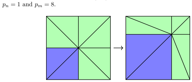
"Thus, the Gibbs phenomenon can be eliminated by taking the limit q→1 provided that the L1(Ω)-best approximation does not exhibit Gibbs phenomena. The results in [5] show that this depends on the mesh that is chosen. [...] From [5] we can infer that the L1-best approximation does not exhibit overshoots if the volume of the green area is smaller or equal to the volume of the blue area."

The paper's conditional Gibbs-elimination claim and its mesh-design rule are both attributed to [5], an unpublished manuscript by the same three authors. The mesh criterion (green area <= blue area) is used to 'predict' and to design meshes on which the method's overshoots vanish, but that criterion is not proved in this paper and no independent external source is supplied. For the specific numerical examples the paper also computes Lq-best approximations directly, so the main method-to-Lq-best comparison retains independent content; however, the general claim and the mesh-design predictions reduce to an unverified same-author citation chain.

full rationale

The paper's own derivation of the nonlinear Petrov-Galerkin method and its quasi-optimality estimate (Sections 3.1-3.3, eqs. (3.10)-(3.12)) is presented with formulas and constants, not by fitting parameters to force a conclusion. The no-overshoot phenomenon is verified against known analytical solutions (Examples 5.1-5.4) and by directly computing Lq-best approximations in Figure 12, so those results are not circular by construction. The main circularity concern is the reliance on [5], an unpublished result by the same authors, for the mesh-dependent behavior of L1-best approximations and for the design of meshes that eliminate Gibbs phenomena. This is a load-bearing same-author citation for the paper's 'prediction' and mesh-design contribution, although it is not a fitted-input or definitional circularity. Hence score 3 rather than a higher score.

Assumptions & free parameters 3 free parameters · 6 assumptions · 0 invented entities

The method introduces no new physical entities. The free parameters are explicit method parameters (q, α, ω) rather than hidden fitted constants; the central numerical claim (vanishing overshoot as q→1) is not obtained by tuning these to match data. The main assumptions are standard functional analysis, the inf-sup result from the authors' earlier work [28], the unproven Fortin condition, and unpublished mesh results [5].

free parameters (3)

q (Lq exponent) = Varied in experiments; focus on q→1 (q=1.01, 1.1)
The central claim concerns the limit q→1; q is a user-chosen parameter of the method, not derived from the problem data.
α (Lq' norm weighting in test norm (4.4)) = 0 or 1 across experiments
Chooses which norm term dominates in ‖·‖_V; affects robustness and quality of approximation (Section 5.2.1).
ω(x) (streamline weighting in test norm) = 0, 1, or x+ε in experiments
Defines the non-standard test norm; used to address robustness and in Section 4.4 to connect with Guermond's L1 method or optimal test norm.

assumptions (6)

standard math Hahn-Banach corollary: the duality map J^φ_V(v) is non-empty for every v (Def. 2.1).
Used in Section 2 to define the duality mapping used throughout the method (eq. 2.1).
standard math Asplund's theorem characterizes the duality map as the subdifferential of ψ(‖·‖) (Thm. 2.3).
Basis for computing duality maps in Section 2.2 and for the mixed formulation.
standard math Milman-Pettis and uniform convexity imply reflexivity and single-valuedness of duality maps (Prop. 2.2).
Ensures the duality map is a well-defined single-valued operator for the spaces considered.
domain assumption Inf-sup condition for Bε on W^{1,q}_0 × W^{1,q'}_0 with robustness constants from [28]; requires c − (1/q)∇·b ≥ c0 > 0 and Poisson regularity.
Invoked in Section 4 to guarantee well-posedness and quasi-best approximation (eq. 3.6); constants are parameter-dependent, so robustness is not assured.
ad hoc to paper Existence of Fortin projector Π: V→Vm satisfying (3.11).
Assumed for the error bound (3.12); the paper states sufficient conditions are 'highly non-trivial' and only numerically observes compatibility for Δp≥2 (Section 5.2.3).
domain assumption Characterization from unpublished [5]: L1-best approximation has no overshoot on certain meshes (e.g., local volume balancing, alignment).
Used in Sections 5.3.2 and 5.3.3 to predict and design meshes that eliminate overshoots as q→1; the result is not publicly available and is from the same authors.

how reviews work

0 comments

Cite this review

Pith. "Pith review of Eliminating Gibbs Phenomena: A Non-linear Petrov-Galerkin Method for the Convection-Diffusion-Reaction Equation." pith.science (2026). https://pith.science/paper/B6LWNLYH

@misc{pith2026190800996,
  author       = {Pith},
  title        = {Pith review of: Eliminating Gibbs Phenomena: A Non-linear Petrov-Galerkin Method for the Convection-Diffusion-Reaction Equation},
  year         = {2026},
  howpublished = {\url{https://pith.science/paper/B6LWNLYH}},
  note         = {Machine review of arXiv:1908.00996}
}

abstract

In this article we consider the numerical approximation of the convection-diffusion-reaction equation. One of the main challenges of designing a numerical method for this problem is that boundary layers occurring in the convection-dominated case can lead to non-physical oscillations in the numerical approximation, often referred to as Gibbs phenomena. The idea of this article is to consider the approximation problem as a residual minimization in dual norms in Lq-type Sobolev spaces, with 1 < q < $\infty$. We then apply a non-standard, non-linear PetrovGalerkin discretization, that is applicable to reflexive Banach spaces such that the space itself and its dual are strictly convex. Similar to discontinuous Petrov-Galerkin methods, this method is based on minimizing the residual in a dual norm. Replacing the intractable dual norm by a suitable discrete dual norm gives rise to a non-linear inexact mixed method. This generalizes the Petrov-Galerkin framework developed in the context of discontinuous Petrov-Galerkin methods to more general Banach spaces. For the convection-diffusion-reaction equation, this yields a generalization of a similar approach from the L2-setting to the Lq-setting. A key advantage of considering a more general Banach space setting is that, in certain cases, the oscillations in the numerical approximation vanish as q tends to 1, as we will demonstrate using a few simple numerical examples.

Figures

Figures reproduced from arXiv: 1908.00996 by the authors.

**Figure 1.** Example 5.2 with ε = 1 and q = 1.2. Convergence for pn = 1 and ∆p = 1, 4, 7. 10 -1 h 10 -12 10 -11 10 -10 10 -9 10 -8 10 -7 10 -6 10 -5 10 -4 10 -3 ||u ¡ u h ||L q 2.87 1 3.95 1 5.11 1 6.05 1 pn = 2 pn = 3 pn = 4 pn = 5 10 -1 h 10 -9 10 -8 10 -7 10 -6 10 -5 10 -4 10 -3 10 -2 ||u ¡ u h ||W 1;q 0 2.07 1 3.14 1 3.85 1 5.04 1 pn = 2 pn = 3 pn = 4 pn = 5 [PITH_FULL_IMAGE:figures/full_fig_p014_1.png] view at source ↗

**Figure 2.** Example 5.2 with ε = 1 and q = 1.2, for pn = 2, 3, 4, 5 and ∆p = 2. Left: L q (Ω)-norm, Right: W1,q (Ω)-norm Example 5.4 (Interior and Boundary Layer). b · ∇u − ε∆u = 0 in (0, 1)2 , u = 1 on ∂Ω ∩ {x = 0}, u = 0 on ∂Ω \ {x = 0}, (5.9) with b = (2, 1)T . For this example, a boundary layer develops at Γ+ ∩ {y > 0.5} and an interior layer along the line y = 0.5x. 5.1 Convergence Tests We start with investigating the con… view at source ↗

**Figure 3.** L q (Ω)-error for Example 5.2 with ε = 10−4 and pn = 1. observe that the error is larger for ∆p = 1. Note that we did not observe this in the diffusive regime. The plot on the right shows that in the convection-dominated regime we obtain a convergence rate of approximately O(h 1 q ) as h tends to zero; this is consistent with the approximation error bound of the piecewise linear interpolant of a jump discontinuity. … view at source ↗

Figures from the paper (13 more)

**Figure 4.** Figure 4: Solution un for q = 2 and q = 1.01 using different norms, i.e., different weighting functions ω(x), and either Dirichlet boundary conditions for r on the whole boundary (strong bc) or weak boundary conditions on r on the inflow boundary and Dirichlet conditions on the …

**Figure 5.** Figure 5: Example 5.1 with ε = 10−5 : Numerical approximations un (left) and rm (right) with a uniform mesh consisting of 8 intervals using piecewise linear polynomials for un and polynomials of degree pm = 10 for rm for varying values of q. Top center: Zoom-in showing over- and…

**Figure 6.** Figure 6: Example 5.1 with ε = 10−6 and q = 1.01, q 0 = 101: Numerical approximations un (left) and rm (right) with a uniform mesh consisting of 8 intervals using piecewise linear polynomials for un and varying polynomial degrees pm for rm. Top center: Zoom-in showing over- and…

**Figure 7.** Figure 7: Example 5.1 with q = 1.01, q 0 = 101: Numerical approximations un (left) and rm (right) with a uniform mesh consisting of 16 intervals using piecewise linear polynomials for un and polynomials of degree pm = 10 for rm for varying values of ε. Top center: Zoom-in showin…

**Figure 8.** Figure 8: Example 5.1 with q = 1.01, q 0 = 101: Numerical approximations un (left) and rm (right) with a uniform mesh consisting of 16 intervals using piecewise linear polynomials for un and polynomials of degree pm = 10 for rm for varying values of ε. Top center: Zoom-in showin…

**Figure 9.** Figure 9: Four Different Meshes on the Unit Square [PITH_FULL_IMAGE:figures/full_fig_p020_9.png]

**Figure 10.** Figure 10: Approximation of the analytical solution of Example 5.2 (Eriksson-Johnson [PITH_FULL_IMAGE:figures/full_fig_p020_10.png]

**Figure 11.** Figure 11: Approximation of the analytical solution of Example 5.2 (Eriksson-Johnson [PITH_FULL_IMAGE:figures/full_fig_p020_11.png]

**Figure 12.** Figure 12: Example 5.2: max(un − uˆ), where ˆu is the interpolant of the analytical solution u in the space Un, for the L q (Ω)-best approximation and the finite element approximations with α = 1 and α = 0. and the approximation for the L q (Ω)-best approximation and the error b…

**Figure 13.** Figure 13: Example 5.3 with b = (2, 1)T : Mesh and approximation for ε = 10−6 with pn = 1 and pm = 8 [PITH_FULL_IMAGE:figures/full_fig_p022_13.png]

**Figure 14.** Figure 14: Modification of Mesh 2: Elements connected to the boundary are marked [PITH_FULL_IMAGE:figures/full_fig_p022_14.png]

**Figure 15.** Figure 15: Example 5.4 with ε = 10−6 . (a) Approximation with q = 2 and b = (2, 1.2)T on Mesh B. (b) Approximation with q = 1.1 and b = (2, 1.2)T on Mesh B. (c) Approximation with q = 2 and b = (2, 1.06)T on Mesh B. (d) Approximation with q = 1.1 and b = (2, 1.06)T on Mesh B [P…

**Figure 16.** Figure 16: Example 5.4 with ε = 10−6 , b = (2, 1.2)T (top) andb = (2, 1.06)T (bottom). 6 Conclusions and Future Directions In this article, we generalized the framework employed for DPG methods to more general Banach spaces. This framework in principle allows us to choose the no…

Discussion (0). Continue with ORCID to comment.

Forward citations

Cited by 1 Pith paper

Reviewed papers in the Pith corpus that reference this work. Sorted by Pith novelty score. Full citation record

Gibbs Phenomena for $L^q$-Best Approximation in Finite Element Spaces -- Some Examples
math.NA 2019-09 conditional novelty 5.0 of 10

On certain 1D and 2D meshes, the Lq-best approximation of a discontinuity in piecewise-linear finite element spaces has over/undershoots that vanish as q tends to 1, while on other meshes they persist even at q=1.

Reference graph

Works this paper leans on

41 extracted references · 39 canonical work pages · cited by 1 Pith paper

[28]

Houston, I

P. Houston, I. Muga, S. Roggendorf, K. G. van der Zee, The Convection- Diﬀusion-Reaction Equation in Non-Hilbert Sobolev Spaces: A Direct Proof of the Inf-Sup Condition and Stability of Galerkin’s Method, Comput. Methods Appl. Math. 19 (3) (2019) 503–522

work page 2019
[5]

Houston, S

P. Houston, S. Roggendorf, K. G. van der Zee, Gibbs Phenomenon for Lq-Best Approximation of Discontinuities in Finite Element Spaces – Some Examples (Unpublished Result)

work page
[1]

J. W. Gibbs, Fourier’s series, Nature 59 (1539) (1899) 606
[2]

Wilbraham, On a certain periodic function, Cambridge and Dublin Math

H. Wilbraham, On a certain periodic function, Cambridge and Dublin Math. J 3 (198) (1848) 1848

work page
[3]

Richards, A Gibbs phenomenon for spline functions, Journal of approximation theory 66 (3) (1991) 334–351

F. Richards, A Gibbs phenomenon for spline functions, Journal of approximation theory 66 (3) (1991) 334–351

work page 1991
[4]

E. B. Saﬀ, S. Tashev, Gibbs phenomenon for bestLp approximation by polygonal lines, East J. Approx. 5 (2) (1999) 235–251. 24

work page 1999
[6]

Moskona, P

E. Moskona, P. Petrushev, E. Saﬀ, The gibbs phenomenon for best L1- trigonometric polynomial approximation, Constructive Approximation 11 (3) (1995) 391–416

work page 1995
[7]

Guermond, A ﬁnite element technique for solving ﬁrst-order PDEs in LP , SIAM J

J.-L. Guermond, A ﬁnite element technique for solving ﬁrst-order PDEs in LP , SIAM J. Numer. Anal. 42 (2) (2004) 714–737

work page 2004

Show all 41 references

[8]

J. E. Lavery, Nonoscillatory solution of the steady-state inviscid Burgers’ equa- tion by mathematical programming, J. Comput. Phys. 79 (2) (1988) 436–448

1988
[9]

J. E. Lavery, Solution of steady-state one-dimensional conservation laws by math- ematical programming, SIAM J. Numer. Anal. 26 (5) (1989) 1081–1089

1989
[10]

J. E. Lavery, Solution of steady-state, two-dimensional conservation laws by mathematical programming, SIAM J. Numer. Anal. 28 (1) (1991) 141–155

1991
[11]

B.-N. Jiang, Non-oscillatory and non-diﬀusive solution of convection problems by the iteratively reweighted least-squares ﬁnite element method, Journal of com- putational physics 105 (1) (1993) 108–121

1993
[12]

Jiang, The least-squares ﬁnite element method: theory and applications in computational ﬂuid dynamics and electromagnetics, Springer Science & Business Media, 1998

B.-N. Jiang, The least-squares ﬁnite element method: theory and applications in computational ﬂuid dynamics and electromagnetics, Springer Science & Business Media, 1998

1998
[13]

Guermond, B

J.-L. Guermond, B. Popov, Linear advection with ill-posed boundary conditions via L1-minimization, Int. J. Numer. Anal. Model. 4 (1) (2007) 39–47

2007
[14]

Guermond, F

J.-L. Guermond, F. Marpeau, B. Popov, A fast algorithm for solving ﬁrst-order PDEs by L1-minimization, Commun. Math. Sci. 6 (1) (2008) 199–216

2008
[15]

Guermond, B

J.-L. Guermond, B. Popov, L1-approximation of stationary Hamilton-Jacobi equations, SIAM J. Numer. Anal. 47 (1) (2008/09) 339–362

2008
[16]

Guermond, B

J.-L. Guermond, B. Popov, An optimal L1-minimization algorithm for stationary Hamilton-Jacobi equations, Commun. Math. Sci. 7 (1) (2009) 211–238

2009
[18]

L. F. Demkowicz, J. Gopalakrishnan, An overview of the discontinuous Petrov Galerkin method, in: Recent developments in discontinuous Galerkin ﬁnite el- ement methods for partial diﬀerential equations, Vol. 157 of IMA Vol. Math. Appl., Springer, Cham, 2014, pp. 149–180

2014
[19]

J. Chan, J. A. Evans, W. Qiu, A dual Petrov-Galerkin ﬁnite element method for the convection-diﬀusion equation, Comput. Math. Appl. 68 (11) (2014)

2014
[20]

Broersen, R

D. Broersen, R. Stevenson, A robust Petrov-Galerkin discretisation of convection- diﬀusion equations, Comput. Math. Appl. 68 (11) (2014) 1605–1618

2014
[21]

Broersen, R

D. Broersen, R. P. Stevenson, A Petrov-Galerkin discretization with optimal test space of a mild-weak formulation of convection-diﬀusion equations in mixed form, IMA J. Numer. Anal. 35 (1) (2015) 39–73

2015
[22]

J. Chan, N. Heuer, T. Bui-Thanh, L. Demkowicz, A robust DPG method for convection-dominated diﬀusion problems II: adjoint boundary conditions and mesh-dependent test norms, Comput. Math. Appl. 67 (4) (2014) 771–795

2014
[23]

Cohen, W

A. Cohen, W. Dahmen, G. Welper, Adaptivity and variational stabilization for convection-diﬀusion equations, ESAIM Math. Model. Numer. Anal. 46 (5) (2012) 1247–1273. 25

2012
[24]

Demkowicz, N

L. Demkowicz, N. Heuer, Robust DPG method for convection-dominated diﬀu- sion problems, SIAM J. Numer. Anal. 51 (5) (2013) 2514–2537

2013
[25]

M. S. Alnæs, J. Blechta, J. Hake, A. Johansson, B. Kehlet, A. Logg, C. Richard- son, J. Ring, M. E. Rognes, G. N. Wells, The FEniCS project version 1.5, Archive of Numerical Software 3 (100) (2015)

2015
[26]

Logg, K.-A

A. Logg, K.-A. Mardal, G. N. Wells, et al., Automated Solution of Diﬀerential Equations by the Finite Element Method, Springer, 2012

2012
[27]

I. Muga, K. G. van der Zee, Discretization of Linear Problems in Banach Spaces: Residual Minimization, Nonlinear Petrov-Galerkin, and Monotone Mixed Meth- ods, arXiv preprint arXiv:1511.04400v1 (2015)

2015 arXiv
[29]

Brezis, Functional analysis, Sobolev spaces and partial diﬀerential equations, Universitext, Springer, New York, 2011

H. Brezis, Functional analysis, Sobolev spaces and partial diﬀerential equations, Universitext, Springer, New York, 2011

2011
[30]

Deimling, Nonlinear functional analysis, Springer-Verlag, Berlin, 1985

K. Deimling, Nonlinear functional analysis, Springer-Verlag, Berlin, 1985

1985
[31]

Zeidler, Nonlinear functional analysis and its applications

E. Zeidler, Nonlinear functional analysis and its applications. III, Springer- Verlag, New York, 1985, variational methods and optimization, Translated from the German by Leo F. Boron

1985
[32]

Cioranescu, Geometry of Banach spaces, duality mappings and nonlinear prob- lems, Vol

I. Cioranescu, Geometry of Banach spaces, duality mappings and nonlinear prob- lems, Vol. 62 of Mathematics and its Applications, Kluwer Academic Publishers Group, Dordrecht, 1990

1990
[33]

Chidume, Geometric properties of Banach spaces and nonlinear iterations, Vol

C. Chidume, Geometric properties of Banach spaces and nonlinear iterations, Vol. 1965 of Lecture Notes in Mathematics, Springer-Verlag London, Ltd., Lon- don, 2009

1965
[34]

Demkowicz, J

L. Demkowicz, J. Gopalakrishnan, Discontinuous Petrov-Galerkin (DPG) method, ICES Report (15–20) (2015)

2015
[35]

Demkowicz, J

L. Demkowicz, J. Gopalakrishnan, A class of discontinuous Petrov-Galerkin methods. II. Optimal test functions, Numer. Methods Partial Diﬀerential Equa- tions 27 (1) (2011) 70–105

2011
[36]

Stakgold, M

I. Stakgold, M. J. Holst, Green’s functions and boundary value problems, Vol. 99, John Wiley & Sons, 2011

2011
[37]

Zitelli, I

J. Zitelli, I. Muga, L. Demkowicz, J. Gopalakrishnan, D. Pardo, V. M. Calo, A class of discontinuous Petrov-Galerkin methods. Part IV: the optimal test norm and time-harmonic wave propagation in 1D, J. Comput. Phys. 230 (7) (2011) 2406–2432

2011
[38]

Gopalakrishnan, W

J. Gopalakrishnan, W. Qiu, An analysis of the practical DPG method, Mathe- matics of Computation 83 (286) (2014) 537–552

2014
[39]

Gopalakrishnan, Five lectures on DPG methods, arXiv:1306.0557 (2013)

J. Gopalakrishnan, Five lectures on DPG methods, arXiv:1306.0557 (2013)

2013 arXiv
[40]

I. Muga, M. J. W. Tyler, K. G. van der Zee, The Discrete-Dual Minimal-Residual Method (DDMRes) for Weak Advection-Reaction Problems in Banach Spaces, Comput. Methods Appl. Math. 19 (3) (2019) 557–579

2019
[41]

Solin, L

P. Solin, L. Korous, P. Kus, Hermes2D, a C++ library for rapid development of adaptive hp-FEM and hp-DG solvers, J. Comput. Appl. Math. 270 (2014) 152–165

2014
[42]

Demkowicz, T

L. Demkowicz, T. F¨ urer, N. Heuer, X. Tian, The double adaptivity paradigm (how to circumvent the discrete inf-sup conditions of babuÅąka and brezzi), ICES Report (19–07) (2019). 26

2019

Pith tools

Reviewed August 14, 2026 · model on record in the stance chip above.

[1] [28]

Houston, I

P. Houston, I. Muga, S. Roggendorf, K. G. van der Zee, The Convection- Diﬀusion-Reaction Equation in Non-Hilbert Sobolev Spaces: A Direct Proof of the Inf-Sup Condition and Stability of Galerkin’s Method, Comput. Methods Appl. Math. 19 (3) (2019) 503–522

work page 2019

[2] [5]

Houston, S

P. Houston, S. Roggendorf, K. G. van der Zee, Gibbs Phenomenon for Lq-Best Approximation of Discontinuities in Finite Element Spaces – Some Examples (Unpublished Result)

work page

[3] [1]

J. W. Gibbs, Fourier’s series, Nature 59 (1539) (1899) 606

[4] [2]

Wilbraham, On a certain periodic function, Cambridge and Dublin Math

H. Wilbraham, On a certain periodic function, Cambridge and Dublin Math. J 3 (198) (1848) 1848

work page

[5] [3]

Richards, A Gibbs phenomenon for spline functions, Journal of approximation theory 66 (3) (1991) 334–351

F. Richards, A Gibbs phenomenon for spline functions, Journal of approximation theory 66 (3) (1991) 334–351

work page 1991

[6] [4]

E. B. Saﬀ, S. Tashev, Gibbs phenomenon for bestLp approximation by polygonal lines, East J. Approx. 5 (2) (1999) 235–251. 24

work page 1999

[7] [6]

Moskona, P

E. Moskona, P. Petrushev, E. Saﬀ, The gibbs phenomenon for best L1- trigonometric polynomial approximation, Constructive Approximation 11 (3) (1995) 391–416

work page 1995

[8] [7]

Guermond, A ﬁnite element technique for solving ﬁrst-order PDEs in LP , SIAM J

J.-L. Guermond, A ﬁnite element technique for solving ﬁrst-order PDEs in LP , SIAM J. Numer. Anal. 42 (2) (2004) 714–737

work page 2004