REVIEW 4 major objections 6 minor 6 references
Fluid Simulation on Vortex Particle Flow Maps
T0 review · 4 major / 6 minor · reviewed 2026-08-07 · deepseek-v4-flash
Pith's one-line read The authors propose VPFM, a hybrid vortex-particle flow-map method that carries vorticity on long particle trajectories and reconstructs velocity on a grid, claiming 3-12x longer flow maps, indefinite 2D stability, and up to 30x longer…
desk verdict Real novelty in on-particle Hessian evolution with strong results, but the NFM ablation and 'indefinitely stable' framing need fixing. read the letter →
The pith
A machine-rendered reading of the paper's core claim, the machinery that carries it, and where it could break.
The reading
What carries the argument
The central object is the particle trajectory used as a bidirectional flow map: each vortex particle carries the forward Jacobian $\mathbf{F}$, the backward Jacobian $\mathbf{T}$, and the flow-map Hessian $\nabla\mathbf{F}$, all updated during RK4 marching. Vorticity is transported as $\boldsymbol{\omega}(\boldsymbol{x},t)=\mathbf{F}_t\,\boldsymbol{\omega}(\boldsymbol{\psi}(\boldsymbol{x}),0)$, the Hessian evolves by the paper's derived evolution equation, and an adaptive split uses a long map $n_L$ for vorticity but a short map $n_S$ for vorticity gradients. Velocity is rebuilt on the grid by solving a vector potential and a harmonic potential with a symmetric positive semi-definite cut-cell system, while no-slip is approximated by a cheap Brinkmann penalization that injects vorticity near solid faces.
What would settle it
Simulate flow around a stationary airfoil or torus with net circulation at Reynolds number around 1000 using VPFM, and compare the time history of lift and shed circulation against a body-fitted direct Navier-Stokes reference; if the unmodeled harmonic component shows up as a systematic drift or divergence, the central long-flow-map claim fails on exactly the geometry class the paper leaves open.
Extended reading notes
Core claim
The paper's claim, stated as a fair reader would report it, is that a vortex method built on particle flow maps can escape the short flow-map lifetimes that have limited prior flow-map methods. The reason is twofold: vorticity reconstruction involves one fewer derivative than impulse or velocity reconstruction, so the transported variable stays bounded longer, and the flow-map Hessian $\nabla\mathbf{F}$ can be evolved consistently on particles instead of interpolated, preventing the gradient blow-up that kills lower-order methods. With those pieces in place, VPFM reports flow-map lengths of 240 in 2D and 60 in 3D, explosion-free leapfrog benchmarks where prior methods fail within seconds, and preservation of linked rings and knots for tens of times longer than those baselines.
Load-bearing premise
The load-bearing assumption is that the harmonic (irrotational, circulation-carrying) part of the velocity can be re-solved at every step as a static potential with no dynamics of its own, an assumption the paper concedes breaks on non-simply-connected domains.
Editorial extensions
If this is right
- The reinitialization interval for vortex quantities can be 3-12 times longer than in prior flow-map methods, reducing the frequency of grid-to-particle transfers and the numerical dissipation they introduce.
- In 2D leapfrog benchmarks the paper reports indefinite stability at a flow map length of 240, where prior methods explode within a few seconds.
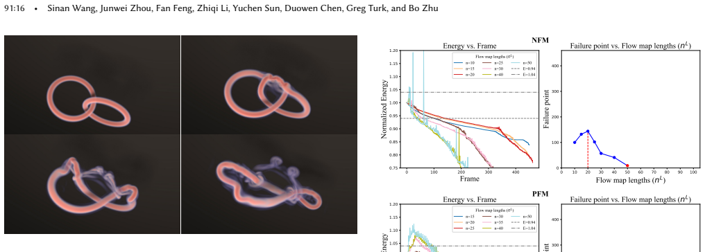
- In the 3D leapfrog benchmark the method preserves separate vortex rings roughly 30 times longer than the neural, particle, and Eulerian vortex flow-map baselines.
- The evolved Hessian term alone about doubles stable simulation time and can be grafted onto the impulse-based PFM method, improving its vortex preservation.
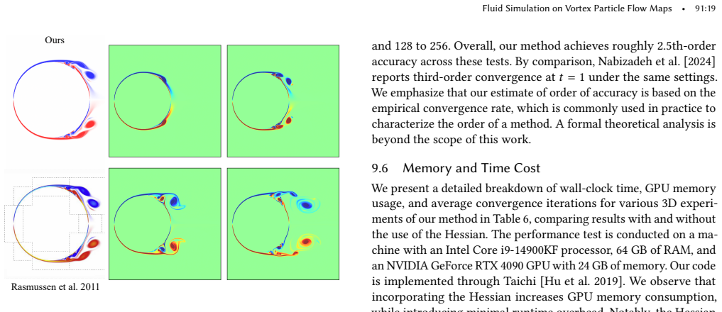
- The cut-cell no-through and Brinkmann-style no-slip treatment allow moving solid boundaries such as propellers and flapping flippers to run with longer flow map lengths than prior methods.
Reading between the lines
- Because the harmonic component's own dynamics are explicitly not modeled, flows with net circulation around obstacles are the most likely place the long-flow-map stability claim breaks; a cohomology-aware coupling would be the natural repair.
- The near-indefinite 2D stability is probably tied to the absence of vortex stretching in 2D, and the paper's own practical cap near $n_L=60$ in 3D suggests stretching-induced blow-up remains the limiting mechanism.
- The simplified Brinkmann penalization has a tunable parameter $\lambda$, so at high Reynolds numbers or fast-moving solids, matching physical vortex shedding may require per-scene calibration that the paper does not address.
- A testable extension would be to run the same Hessian-evolution scheme with a grid-free velocity reconstruction to see whether the grid solve or the particle evolution is the main stabilizer.
Editorial analysis
A structured set of objections, weighed in public.
Referee Report
Summary. The paper proposes VPFM, a hybrid Eulerian-Lagrangian method that carries vorticity, vorticity gradients, flow-map Jacobians, and a flow-map Hessian on vortex particles, while reconstructing velocity on a grid using a vector-potential solve plus a cut-cell harmonic solve. It introduces a novel Hessian evolution equation for particle flow maps, an SPSD cut-cell no-through treatment, and a simplified Brinkmann penalization for approximate no-slip. The central claims are 3-12x longer flow maps than NFM/PFM/EVM and up to 30x longer vorticity preservation in 3D, together with visual examples (leapfrog, Hopf link, trefoil, plesiosaur, propeller, aircraft) and quantitative validations including lid-driven cavity against Ghia et al. and a Taylor-Green convergence study.
Significance. If the long-flow-map claims hold, VPFM is a meaningful advance for vortex methods in graphics: it addresses the known dissipation of VIC while retaining grid-based Poisson solves, and the Hessian evolution and cut-cell harmonic system are novel, well-motivated components. The ablation in Fig. 23 shows the Hessian term extends the stable flow-map length in 3D, and the lid-driven-cavity and Taylor-Green experiments provide falsifiable quantitative checks. However, the headline 3-12x and 30x comparisons are weakened by the use of an ablated NFM baseline and by the unsupported 'indefinitely stable' wording. The significance at the claimed level is therefore not yet established.
major comments (4)
- [§9.1.2, Table 4] The 3-12x flow-map-length advantage is measured against an NFM implementation with the neural buffer removed, as the Table 4 note states: 'For a fair comparison, we implemented an NFM version without the neural buffer and observed that n_L = 20 caused the 2D leapfrog simulation to explode.' The neural buffer is a core NFM component that corrects flow-map error accumulation; an ablated NFM is not the state-of-the-art method the paper claims to outperform. Please report the intact NFM's maximum stable n_L for the 2D leapfrog and trefoil cases (or justify quantitatively why the ablation does not affect the comparison), and temper the '3-12x' and '30x' claims accordingly.
- [§1 and Table 3] The statement that the method 'remains indefinitely stable in 2D benchmarks' is an extrapolation from a run to 600 s (the text in §9.1.2 reports 613 s before merging), not a proof or a long-time numerical demonstration. Table 3 lists '∞' for the 2D explosion time, but the simulation was terminated at finite time. Please replace 'indefinitely stable' and the '∞' entry with the finite simulated duration, or provide a genuine long-time stability analysis or a mathematical argument.
- [§11, §12, and §3.2] The velocity reconstruction assumes the harmonic component u_h is the gradient of a scalar harmonic function satisfying the instantaneous no-through condition (Eqs. (4)-(7)), while Section 11 acknowledges that 'the exact harmonic component's dynamics are not accounted for.' On non-simply-connected domains or with moving boundaries, the harmonic component can carry its own circulation and advective dynamics, which is a correctness risk for the dynamic-boundary examples (plesiosaur, propeller) and for geometries where cohomology matters. Since the limitation is explicitly stated, please quantify its effect on at least one benchmark (e.g., a comparison with a method that couples the harmonic dynamics, such as Yin et al. 2023a, or a test with a known circulation) or restrict the claims to settings where this approximation is controlled.
- [§9.1.1, Table 3] The '30x longer' claim in 3D is obtained by forcing all methods to n_L = 100, far beyond the optimal n_L = 20 for NFM and n_L = 20-30 for the other baselines. Stress-testing at a common long flow map is informative, but this operating point is outside the baselines' designed regime, so the ratio is not a neutral measure of practical advantage. Please present the same comparison at each method's recommended n_L (Table 4 partially does this) and clearly distinguish the 'robust to over-long flow maps' claim from the 'practical long-flow-map advantage' claim.
minor comments (6)
- [§9.1.2 and Fig. 15] The text reports '613 seconds before merging' for the 2D leapfrog, while Figure 15 and Table 3 use '600s' and '∞'; please make the termination time and the definition of 'merge' consistent.
- [§9.1.2] 'Through theseventh leap' should read 'through the seventh leap' (missing space).
- [Figures 22, 28, 30] The figure labels in the supplied text appear as unicode placeholder glyphs such as '/uni00000013'; please ensure the final PDF renders all axis labels and legend text correctly.
- [Eq. (13)] Eq. (13) uses the tensor product ∇F_t ω before the index contraction is explained; please define the contraction explicitly before or at Eq. (13) rather than only in the sentence after it.
- [§5.4] The Monte Carlo fluid-fraction sampling should state the number of samples per face and, ideally, provide a short convergence test for the fluid fraction estimation.
- [Algorithm 3] Algorithm 3 lists ω^g_c as both an input and an output, but the accompanying description only explains the update to ω^p_a; please clarify the return convention.
Circularity Check
No significant circularity: the central stability and vorticity-preservation claims are empirical outcomes validated against external benchmarks, and self-citations are not load-bearing.
full rationale
The paper's core derivation chain is self-contained. The vorticity transport law (Eq. 12) and the vorticity gradient evolution (Eq. 13) follow from standard flow-map kinematics cited to Cortez (1995), and the novel Hessian evolution (Eq. 14) is obtained by differentiating the known Jacobian evolution (Eq. 11), with the derivation deferred to the supplementary material rather than assumed from prior work. The long flow-map capability is demonstrated empirically: the flow-map length nL is a user-set parameter, and the paper reports explosion times and vortex-structure preservation without fitting any parameter to reproduce the leapfrog or trefoil results. The claimed 3-12x and 30x improvements are therefore measured outcomes, not quantities defined in terms of the baselines. The paper does rely heavily on the authors' own NFM, PFM, and EVM flow-map methods as baselines and as motivation, but this is normal self-citation rather than circularity: the baselines are implemented and run, and independent grounding is provided by analytic Taylor-Green convergence, the Ghia et al. (1982) lid-driven cavity benchmark, and agreement with Villois et al. (2020) on the Hopf link. The removal of NFM's neural buffer for a 'fair comparison' (Table 4) is a legitimate benchmarking concern that could affect the size of the reported advantage, but it does not make the VPFM result equivalent to its inputs by construction; it is a correctness/comparability issue, not a circularity issue. The acknowledged harmonic-component limitation (Section 11) likewise reflects an unmodeled dynamics term, not a circular definition. No equation in the paper reduces to its own output, and no fitted parameter is renamed as a prediction.
Assumptions & free parameters
free parameters (5)
- n_L (long flow map length) =
60 in 3D, 240 in 2D leapfrog
- n_S (short flow map length) =
1
- lambda (Brinkmann penalization coefficient) =
1/delta_t for static solids, 1/(100 delta_t) to 1/(2 delta_t) for moving solids
- CFL number =
0.5 (3D), 1.0 (2D)
- fluid fraction threshold alpha =
0.1
assumptions (4)
- domain assumption Incompressible Navier-Stokes equations and their vorticity form (Eq. 3)
- standard math Vorticity transport as a 2-form: omega(x,t)=F omega0(psi(x)) (Eq. 12)
- ad hoc to paper Helmholtz decomposition of velocity into solenoidal and harmonic parts with the harmonic part as gradient of a scalar potential (Eq. 4-7)
- domain assumption Velocity second derivatives (grad grad u) are well-resolved by grid finite differences and can be interpolated to particles for Hessian evolution (Eq. 14)
Cite this review
Pith. "Pith review of Fluid Simulation on Vortex Particle Flow Maps." pith.science (2026). https://pith.science/paper/BCM22G3M
@misc{pith2026250521946,
  author       = {Pith},
  title        = {Pith review of: Fluid Simulation on Vortex Particle Flow Maps},
  year         = {2026},
  howpublished = {\url{https://pith.science/paper/BCM22G3M}},
  note         = {Machine review of arXiv:2505.21946}
}
read the original abstract
We propose the Vortex Particle Flow Map (VPFM) method to simulate incompressible flow with complex vortical evolution in the presence of dynamic solid boundaries. The core insight of our approach is that vorticity is an ideal quantity for evolution on particle flow maps, enabling significantly longer flow map distances compared to other fluid quantities like velocity or impulse. To achieve this goal, we developed a hybrid Eulerian-Lagrangian representation that evolves vorticity and flow map quantities on vortex particles, while reconstructing velocity on a background grid. The method integrates three key components: (1) a vorticity-based particle flow map framework, (2) an accurate Hessian evolution scheme on particles, and (3) a solid boundary treatment for no-through and no-slip conditions in VPFM. These components collectively allow a substantially longer flow map length (3-12 times longer) than the state-of-the-art, enhancing vorticity preservation over extended spatiotemporal domains. We validated the performance of VPFM through diverse simulations, demonstrating its effectiveness in capturing complex vortex dynamics and turbulence phenomena.
Figures


Figures from the paper (25 more)







Reference graph
Works this paper leans on
-
[2001]
Marcel Padilla, Albert Chern, Felix Knöppel, Ulrich Pinkall, and Peter Schröder
Blending finite-difference and vortex methods for incompressible flow com- putations.SIAM Journal on Scientific Computing22, 5 (2001), 1655–1674. Marcel Padilla, Albert Chern, Felix Knöppel, Ulrich Pinkall, and Peter Schröder. 2019. On bubble rings and ink chandeliers.ACM Transactions on Graphics (TOG)38, 4 (2019), 1–14. Sang Il Park and Myoung Jun Kim. 2...
2001
-
[2015]
Nicholas K-R Kevlahan and Jean-Michel Ghidaglia
The affine particle-in-cell method.ACM Transactions on Graphics (TOG)34, 4 (2015), 1–10. Nicholas K-R Kevlahan and Jean-Michel Ghidaglia. 2001. Computation of turbulent flow past an array of cylinders using a spectral method with Brinkman penalization. European Journal of Mechanics-B/Fluids20, 3 (2001), 333–350. ByungMoon Kim, Yingjie Liu, Ignacio Llamas,...
arXiv 2015
-
[2016]
Schrödinger’s smoke.ACM Transactions on Graphics (TOG)35, 4 (2016), 1–13. Alexandre Joel Chorin. 1973. Numerical study of slightly viscous flow.Journal of fluid mechanics57, 4 (1973), 785–796. Alexandre Joel Chorin. 1978. Vortex sheet approximation of boundary layers.Journal of computational physics27, 3 (1978), 428–442. Alexandre Joel Chorin. 1980. Vorte...
work page 2016
-
[2019]
Markus Ihmsen, Jens Orthmann, Barbara Solenthaler, Andreas Kolb, and Matthias Teschner
Taichi: a language for high-performance computation on spatially sparse data structures.ACM Transactions on Graphics (TOG)38, 6 (2019), 1–16. Markus Ihmsen, Jens Orthmann, Barbara Solenthaler, Andreas Kolb, and Matthias Teschner. 2014. SPH fluids in computer graphics. (2014). Sadashige Ishida, Chris Wojtan, and Albert Chern. 2022. Hidden degrees of freedo...
work page 2019
-
[2021]
A Characteristic Mapping method for the two-dimensional incompressible Euler equations.J. Comput. Phys.424 (2021), 109781. Xi-Yuan Yin, Kai Schneider, and Jean-Christophe Nave. 2023b. A Characteristic Mapping Method for the three-dimensional incompressible Euler equations.J. Comput. Phys. (2023), 111876. Xinxin Zhang and Robert Bridson. 2014. A PPPM fast ...
work page 2021
-
[2022]
Yen Ting Ng, Chohong Min, and Frédéric Gibou
Covector fluids.ACM Transactions on Graphics (TOG)41, 4 (2022), 1–16. Yen Ting Ng, Chohong Min, and Frédéric Gibou. 2009. An efficient fluid–solid coupling algorithm for single-phase flows.J. Comput. Phys.228, 23 (2009), 8807–8829. Mohamed Lemine Ould-Salihi, Georges-Henri Cottet, and Mohammed El Hamraoui
work page 2022
Reviewed August 7, 2026 · model on record in the stance chip above.
Discussion (0). Sign in to comment.