REVIEW 4 major objections 6 minor 35 references
Improved Monitoring of Honey bee Colony Strength via Audio IoT Sensors, Modulation Tensorgrams and Recurrent Neural Networks
T0 review · 4 major / 6 minor · reviewed 2026-08-01 · deepseek-v4-flash
Pith's one-line read Keeping the time axis in a modulation spectrogram—a 'modulation tensorgram'—lets deep audio models predict honey-bee colony strength more accurately and generalize across hives than standard spectrograms or MFCCs.
desk verdict Feeding raw modulation tensorgrams to deep nets gives a clear accuracy gain over spectrogram/MFCC baselines on UrBAN; the main weakness is that interpolated labels leave a seasonal-confounding hole that needs a sensitivity analysis. read the letter →
The pith
A machine-rendered reading of the paper's core claim, the machinery that carries it, and where it could break.
The reading
What carries the argument
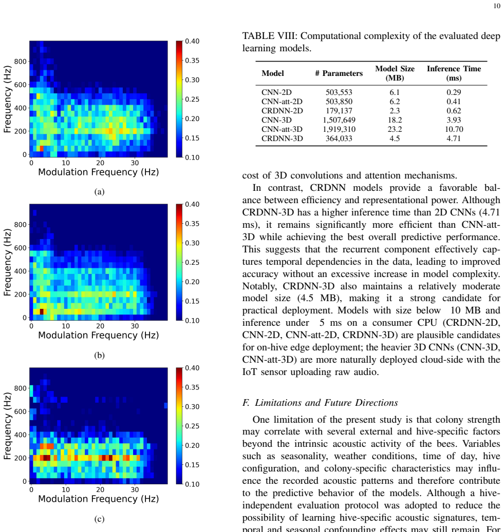
The modulation tensorgram: a 3D array (acoustic frequency × modulation frequency × time) computed by taking a short-time Fourier transform of the audio, then a second STFT along the time axis of each frequency bin, with the time axis preserved instead of averaged away. This is the object that carries the argument: it provides deep networks with both spectral structure and temporal evolution, and the paper's F-ratio analysis identifies which frequency-modulation regions are most discriminative across colony-strength categories.
What would settle it
Compute the model's prediction error separately for segments recorded close to manual inspections versus far from them: if error rises systematically with time since the nearest inspection, the model is tracking interpolated labels. Alternatively, retrain with explicit time-of-day and calendar features and see whether the modulation tensorgram still improves correlation beyond those covariates; if it does not, the temporal dynamics may be seasonal rather than acoustic.
Extended reading notes
Core claim
The central discovery is that modulation-spectrum temporal dynamics are discriminative for honey-bee colony strength and that a modulation tensorgram—a 3D representation of acoustic frequency, modulation frequency, and time—lets deep networks exploit them. In hive-independent evaluation, where entire hives are held out, the best model (a convolutional-recurrent network with 3D tensorgram input) achieves mean absolute error 3.31±1.36 and Pearson correlation r=0.78±0.17, while spectrogram and MFCC baselines stay around r≈0.5. In random splits, the same model reaches MAE 1.01±0.08 and r=0.97±0.01. The paper further shows that the modulation-based inputs benefit less from spectral-subtraction pr
Load-bearing premise
The paper assigns every 15-minute audio segment a colony-strength label by linearly interpolating manual 'frames of bees' counts between sparse inspections (Section III-A), and it acknowledges in Section IV-F that seasonality and environmental factors may confound the acoustic signal; if true colony strength changes nonlinearly between inspections, or if the interpolation mostly encodes time-of-year trends, the reported accuracy and cross-hive gains could partly measure track
Editorial extensions
If this is right
- Hive-strength monitoring could shift from sparse manual inspections to continuous acoustic estimates with errors around one frame of bees in familiar settings and about three frames on entirely unseen hives.
- Models trained on modulation tensorgrams transfer to new hives better than spectrogram or MFCC models, which matters for deploying a single system across many apiaries.
- Because the representation tolerates background noise without aggressive preprocessing, in-the-wild deployments may require less audio enhancement.
- The best-performing recurrent model is light enough (roughly 4.5 MB and a few milliseconds of inference on a consumer CPU) to make on-hive edge deployment plausible.
Reading between the lines
- The largest numerical gap over baselines appears in random splits, where temporally adjacent segments share acoustic conditions; the more meaningful result is the hive-independent gap, and that gap is smaller in absolute terms, so deployment claims should be weighed against the hive-independent numbers.
- A concrete stress test of the interpolation assumption: evaluate prediction error as a function of time since the nearest manual inspection; if errors grow sharply with distance from inspections, the model is partly tracking a linearly interpolated label curve rather than true colony strength.
- Another test: add time-of-day, date, and weather as auxiliary inputs and check whether the tensorgram still adds predictive value; this would separate acoustic temporal dynamics from seasonal confounding, which the paper acknowledges as a remaining limitation.
- The same tensorgram architecture could transfer to other bioacoustic monitoring tasks—such as varroa infestation or queen presence—especially if datasets with per-segment noise annotations become available to test robustness directly.
Signed reviews
Editorial analysis
A structured set of objections, weighed in public.
Referee Report
Summary. The paper proposes a new audio representation for honey bee colony strength estimation: the modulation tensorgram, which retains the time axis of the modulation spectrum instead of averaging it away. Using the public UrBAN dataset (nine hives, two years, over 3,000 hours of audio), the authors feed spectrograms, MFCCs, modulation spectrograms, and modulation tensorgrams into a family of CNN/CRDNN architectures and evaluate them under both random 5-fold splits and hive-independent 5-fold splits. They report that modulation-based inputs consistently outperform spectrogram/MFCC baselines, with the best model (CRDNN-3D on the tensorgram) reaching MAE 1.01±0.08 and r≈0.97 in the random-split setting and MAE 3.31±1.36 and r=0.78±0.17 in the hive-independent setting, versus r≈0.5 for the baselines. The paper also includes Friedman/Nemenyi statistical tests, saliency and Grad-CAM analyses, a comparison with a random-forest baseline, and a computational-complexity assessment. The central claim is that the temporal dynamics of the modulation spectrum carry colony-strength information that static spectral or cepstral features discard.
Significance. If the reported results hold, the paper would make a useful contribution to precision apiculture and to the broader literature on modulation-spectral representations for acoustic monitoring. The strengths of the study are its use of a public, longitudinal dataset; the inclusion of a hive-independent evaluation protocol that is more realistic for deployment; and the transparent reporting of multiple architectures, statistical tests, and computational costs. The main comparison—modulation-based inputs outperforming spectrogram/MFCC inputs in the hive-independent split—is the kind of empirical evidence that could move the field toward richer time-preserving representations. However, the central empirical claim is currently threatened by a label-construction issue: colony-strength labels are linearly interpolated between sparse manual inspections. Because interpolated labels are smooth functions of calendar time, and because all hives share the same seasonal calendar, the reported cross-hive correlation gains could partly reflect tracking of a seasonal/time trend rather than acoustic discrimination of true colony strength. The paper acknowledges seasonal confounding in Section IV-F but
major comments (4)
- [IV-F] The label for every 15-minute audio segment is obtained by linear temporal interpolation between sparse manual inspections (Section III-A). The resulting target is a piecewise-linear, smooth function of calendar time. In the hive-independent split, all hives share the same seasonal calendar, so a model could achieve high correlation by recognizing time-of-year acoustic cues (ambient noise, insect activity, weather-correlated sounds) and predicting the interpolated trend, without estimating frames-of-bees. Section IV-F acknowledges that 'temporal and seasonal confounding effects may still remain,' but no sensitivity analysis is provided. To support the load-bearing claim that modulation temporal dynamics carry colony-strength information, please add at least one of the following controls: (a) a time-only baseline (e.g., day-of-year, or a smoothed inspection curve) compared directly with t
- [II-A/II-B] Several modulation-specific design choices were made empirically on the UrBAN data: the STFT window/hop lengths (100 ms/12.5 ms), the second-stage 60 s window, the 1 kHz frequency cap, and the bin-merging geometry. Section II-A states these were 'optimized empirically based on pilot experimentation,' and Section II-B uses the same dataset's labels to justify the 1 kHz cap and bin geometry. If these choices were tuned on the same data that is later used for evaluation, the comparison against spectrogram/MFCC baselines is optimistically biased in favor of the modulation representation. Please clarify whether all such choices were fixed before model evaluation, e.g., by selecting them on training folds only or on a separate development set, and ideally report sensitivity of the main hive-independent results to these choices (e.g., 50/100/200 ms window, 30 s vs 5 min aggregation). If the cho
- [Table VI] The Friedman average ranks in Table VI contain a clear error: under Random-Split, the MAE ranks are identical for every model between 'No pre-processing' and 'Spectral amplitude subtraction' (e.g., Spec-CNN-2D 6.6/6.6, CRDNN-3D 1.4/1.4, and all other entries), while the corresponding r ranks differ. This duplication is implausible because spectral subtraction changes the input and the MAE values in Table IV. Since the Friedman/Nemenyi analysis is used to support the recommendation of CRDNN-3D, please correct the table, recompute the CD diagrams, and report whether the ranks are pooled over the four scenarios or computed separately. If the corrected ranks alter the statistical conclusions (e.g., if CRDNN-3D no longer separates from the modulation-spectrogram group), revise the claims in Section IV-A accordingly.
- [IV-B] The statistical comparison is reported only as average ranks across the five folds, without confidence intervals or a direct treatment of the fact that the Friedman test is computed on ranks from the same data used to select hyperparameters. More importantly, the Nemenyi CD diagrams in Figure 5 are the main support for the claim that the proposed method is significantly better than the baselines in the hive-independent setting, but the diagrams appear to group most modulation-based methods together. Please clarify whether the claimed advantage of CRDNN-3D over all baselines is statistically significant after correcting Table VI, and report the actual Friedman/Nemenyi p-values for the pairwise comparisons that are highlighted in the text.
minor comments (6)
- [II-A] The description of the tensor dimensions is confusing. The paper states that after the two STFT stages the tensor is (801×801×14), but with a 60 s no-overlap window and 15-minute segments one would expect 15 frames rather than 14. Please clarify the frame count and whether the second-stage window covers the full segment length or is computed with a leftover partial frame.
- [III-A] Figure 4 shows inspection measurements over time, but it is not indicated which points correspond to actual manual inspections and which are interpolated. Please add markers or a note explaining that the plotted curves are the interpolated labels used for training.
- [IV-D] In Table VII the abbreviation 'MSAB' (presumably 'Modulation Spectral Analysis Baseline') is undefined. Please spell it out in the caption or text.
- [IV-A] The text says 'the modulation-based methods are capable of reducing the MAE to around 1.5' in the random-split setting, but Table IV shows a range from 1.01 to 1.61. Please use a range or a representative value to avoid overstating the improvement.
- [IV-E] The inference times are measured on a MacBook Pro with an Apple M1 chip, but the paper does not specify the software/version or whether the timings are CPU-only. Since the deployment discussion depends on these numbers, please provide the measurement conditions and, if possible, report on an edge-class CPU as well.
- [General] The notation for the target variable is inconsistent: 'frames of bees (fob)', 'fobs', and 'fob' are all used. Define the abbreviation once and use it consistently.
Circularity Check
No significant circularity: the central claim is an empirical benchmark against external baselines, and no prediction reduces to its input by construction.
full rationale
The paper's central claim is empirical rather than derivational. Modulation spectrograms/tensorgrams are computed from audio via two STFT stages (Section II-A), while the target fob labels come from manual inspections with linear temporal interpolation (Section III-A). No equation defines the representation in terms of the target, and the reported MAE/r values are not obtained by re-inserting fitted labels. The main comparisons use standard external baselines (spectrogram, MFCC) and held-out hive splits, so the central result has independent empirical content. Self-citations to [27], [29], and [31] supply prior feature definitions, the modulation-spectral framework, and the public UrBAN dataset; none is invoked as a uniqueness theorem or as a substitute for the experiments reported here. Section IV-F explicitly acknowledges residual temporal/seasonal confounding and the absence of per-segment noise annotations; these are limitations on causal interpretation, not evidence that a prediction reduces to an input. The empirically tuned STFT window lengths and the F-ratio-motivated frequency cap (Sections II-A and II-B) raise data-selection/optimism concerns on the same dataset, but that is not the kind of definitional or self-citation circularity this pass is asked to identify.
Assumptions & free parameters
free parameters (3)
- STFT window / hop lengths (100 ms / 12.5 ms) =
100 ms, 12.5 ms
- Second-stage modulation window (60 s, no overlap) =
60 s
- Frequency cap and bin merging geometry =
1 kHz cap; 20 acoustic × 40 modulation bins
assumptions (4)
- domain assumption Linear interpolation of fobs between manual inspections yields a valid continuous colony-strength target.
- domain assumption Colony-strength-relevant acoustic information lies below 1 kHz and is captured by modulation rates resolvable with a 60 s second-stage window.
- domain assumption Spectral amplitude subtraction denoises baseline features without biasing the comparison against modulation-based inputs.
- standard math Standard supervised deep-learning assumptions (loss minimization, early stopping, random and held-out splits) apply to the regression task.
Cite this review
Pith. "Pith review of Improved Monitoring of Honey bee Colony Strength via Audio IoT Sensors, Modulation Tensorgrams and Recurrent Neural Networks." pith.science (2026). https://pith.science/paper/BFV6W3WM
@misc{pith2026260720386,
  author       = {Pith},
  title        = {Pith review of: Improved Monitoring of Honey bee Colony Strength via Audio IoT Sensors, Modulation Tensorgrams and Recurrent Neural Networks},
  year         = {2026},
  howpublished = {\url{https://pith.science/paper/BFV6W3WM}},
  note         = {Machine review of arXiv:2607.20386}
}
read the original abstract
Honey bees (Apis mellifera) play a crucial role in agriculture and ecosystem stability as key pollinators of crops and wild plants. As such, monitoring hive strength remotely with Internet of Things (IoT) sensors has become a crucial task. Previously, handcrafted features extracted from the modulation spectrum of audio IoT devices were shown to improve acoustic monitoring of colony strength. In this paper, we hypothesize that important discriminative information is present in the temporal dynamics of the modulation spectrum, but this information is discarded with prior methods. As such, we explore the use of a new modulation tensorgram where the time dimension is kept. This new representation is used as input to a convolutional neural network (CNN) and a convolutional recurrent deep neural networks (CRDNN). Using the public UrBAN dataset, which contains more than 3,000 hours of beehive audio recordings, we show that the proposed method improves both accuracy and cross-hive generalizability over prior benchmark methods, and the results further suggest improved robustness to noisy in-the-wild recording conditions. We use saliency maps and gradient-weighted class activation maps for explainability and show the importance of the modulation spectral temporal dynamics for the task at hand. Overall, our results suggest that accurate, generalizable, and robust acoustic monitoring of honey bee colony strength is possible.
Figures


Figures from the paper (5 more)



Reference graph
Works this paper leans on
-
[1]
& Others 12 Safeguarding pollinators and their values to human well-being.Nature
Potts, S., Imperatriz-Fonseca, V ., Ngo, H., Aizen, M., Biesmeijer, J., Breeze, T., Dicks, L., Garibaldi, L., Hill, R., Settele, J. & Others 12 Safeguarding pollinators and their values to human well-being.Nature. 540, 220-229 (2016)
2016
-
[2]
& Rana, A
Singh, G. & Rana, A. Honeybees and colony collapse disorder: under- standing key drivers and economic implications.Proceedings Of The Indian National Science Academy. pp. 1-17 (2025)
2025
-
[3]
& Tiwari, R
Mahankuda, B. & Tiwari, R. Impact of Climate Change on Honeybees and Crop Production.Adapting To Climate Change In Agriculture- Theories And Practices: Approaches For Adapting To Climate Change In Agriculture In India. pp. 211-224 (2024)
2024
-
[4]
& Others Threats to an ecosystem service: pressures on pollinators.Frontiers In Ecology And The Environment.11, 251-259 (2013)
Vanbergen, A., Initiative, I. & Others Threats to an ecosystem service: pressures on pollinators.Frontiers In Ecology And The Environment.11, 251-259 (2013)
2013
-
[5]
& Meitalovs, J
Zacepins, A., Stalidzans, E. & Meitalovs, J. Application of information technologies in precision apiculture.Proceedings Of The 13th Interna- tional Conference On Precision Agriculture.7(2012)
2012
-
[6]
& Vella, A
Alleri, M., Amoroso, S., Catania, P., Verde, G., Orlando, S., Ragusa, E., Sinacori, M., Vallone, M. & Vella, A. Recent developments on precision beekeeping: A systematic literature review.Journal Of Agriculture And Food Research.14pp. 100726 (2023)
2023
-
[7]
& Jiang, J
Chen, S., Wang, J., Lin, H., Lee, M., Liu, A., Wu, Y ., Hsu, P., Yang, E. & Jiang, J. A machine learning-based multiclass classification model for bee colony anomaly identification using an IoT-based audio monitoring system with an edge computing framework.Expert Systems With Applications. pp. 124898 (2024)
2024
-
[8]
& Riente, F
Barbisan, L., Turvani, G. & Riente, F. A Machine Learning Approach for Queen Bee Detection Through Remote Audio Sensing to Safeguard Honeybee Colonies.IEEE Transactions On AgriFood Electronics. (2024)
2024
Show all 35 references
-
[9]
& Richard, F
Hunt, J. & Richard, F. Intracolony vibroacoustic communication in social insects.Insectes Sociaux.60, 403-417 (2013)
2013
-
[10]
& Guerrero-M ´endez, C
Robles-Guerrero, A., G ´omez-Jim´enez, S., Saucedo-Anaya, T., L ´opez- Betancur, D., Navarro-Sol ´ıs, D. & Guerrero-M ´endez, C. Convolutional Neural Networks for Real Time Classification of Beehive Acoustic Patterns on Constrained Devices.Sensors.24, 6384 (2024)
2024
-
[11]
& Ashraf, I
Rustam, F., Sharif, M., Aljedaani, W., Lee, E. & Ashraf, I. Bee detection in bee hives using selective features from acoustic data.Multimedia Tools And Applications.83, 23269-23296 (2024)
2024
-
[12]
& Leppard, M
Qandour, A., Ahmad, I., Habibi, D. & Leppard, M. Remote Beehive Monitoring Using Acoustic Signals.Acoustics Australia.42, 205 (2014)
2014
-
[13]
& Falk, T
Abdollahi, M., Zhu, Y ., Guimar ˆaes, H., Coallier, N., Maucourt, S., Giovenazzo, P. & Falk, T. On the Prediction of Varroa Mite Infestations in Honeybee Colonies via Acoustic Monitoring.IEEE Sensors Journal. pp. 1-1 (2026)
2026
-
[14]
& Hotho, A
Janetzky, P., Schaller, M., Krause, A. & Hotho, A. Swarming Detection in Smart Beehives Using Auto Encoders for Audio Data.2023 30th International Conference On Systems, Signals And Image Processing (IWSSIP). pp. 1-5 (2023)
2023
-
[15]
& Falk, T
Zhu, Y ., Abdollahi, M., Maucourt, S., Coallier, N., Guimar ˜aes, H., Giovenazzo, P. & Falk, T. Early prediction of honeybee hive winter sur- vivability using multi-modal sensor data.IEEE International Workshop On Metrology For Agriculture And Forestry. pp. - (2023)
2023
-
[16]
& Falk, T
Zhu, Y ., Abdollahi, M., Maucourt, S., Coallier, N., Guimar ˜aes, H., Giovenazzo, P. & Falk, T. MSPB: a longitudinal multi-sensor dataset with phenotypic trait measurements from honey bees.Scientific Data. 11, 860 (2024)
2024
-
[17]
& Falk, T
Abdollahi, M., Henry, E., Giovenazzo, P. & Falk, T. The importance of context awareness in acoustics-based automated beehive monitoring. Applied Sciences.13, 195 (2022)
2022
-
[18]
& Phan, N
Mattila, H., Kernen, H., Otis, G., Nguyen, L., Pham, H., Knight, O. & Phan, N. Giant hornet (Vespa soror) attacks trigger frenetic antipredator signalling in honeybee (Apis cerana) colonies.Royal Society Open Science.8(2021)
2021
-
[19]
& Logof ˘atu, D
Cejrowski, T., Szyma ´nski, J. & Logof ˘atu, D. Buzz-based recognition of the honeybee colony circadian rhythm.Computers And Electronics In Agriculture.175pp. 105586 (2020)
2020
-
[20]
& Duran, O
Ruvinga, S., Hunter, G., Nebel, J. & Duran, O. Prediction of honeybee swarms using audio signals and convolutional neural networks.Work- shops At 18th International Conference On Intelligent Environments (IE2022). pp. 146-154 (2022)
2022
-
[21]
& Amlathe, P
Kulyukin, V ., Mukherjee, S. & Amlathe, P. Toward audio beehive monitoring: Deep learning vs. standard machine learning in classifying beehive audio samples.Applied Sciences.8, 1573 (2018)
2018
-
[22]
& Pham- Hong, T
Phan, T., Nguyen-Doan, D., Nguyen-Huu, D., Nguyen-Van, H. & Pham- Hong, T. Investigation on new Mel frequency cepstral coefficients fea- tures and hyper-parameters tuning technique for bee sound recognition. Soft Computing.27, 5873-5892 (2023)
2023
-
[23]
& Falk, T
Abdollahi, M., Giovenazzo, P. & Falk, T. Automated beehive acoustics monitoring: A comprehensive review of the literature and recommenda- tions for future work.Applied Sciences.12, 3920 (2022)
2022
-
[24]
& Benetos, E
Nolasco, I., Terenzi, A., Cecchi, S., Orcioni, S., Bear, H. & Benetos, E. Audio-based identification of beehive states.ICASSP 2019-2019 IEEE International Conference On Acoustics, Speech And Signal Processing (ICASSP). pp. 8256-8260 (2019)
2019
-
[25]
& Simons-Rudolph, A
Campell, C., Parry, R., Tashakkori, R., Somer, A., Richardson, L. & Simons-Rudolph, A. Honey Bee Piping Detection Utilizing Convolu- tional Neural Networks.IEEE Sensors Journal. (2025)
2025
-
[26]
& Heo, T
Kim, J., Oh, J. & Heo, T. Acoustic Scene Classification and Visualization of Beehive Sounds Using Machine Learning Algorithms and Grad- CAM.Mathematical Problems In Engineering.2021(2021)
2021
-
[27]
& Falk, T
Abdollahi, M., Zhu, Y ., Guimar ˜aes, H., Coallier, N., Maucourt, S., Giovenazzo, P. & Falk, T. Audio Modulation Spectral Features for Im- proved Honeybee Colony Population Prediction.IEEE Sensors Journal. pp. 1-1 (2025)
2025
-
[28]
& Floquet, R
Bricout, A., Leleux, P., Acco, P., Escriba, C., Fourniols, J., Soto-Romero, G. & Floquet, R. Bee together: Joining bee audio datasets for hive extrapolation in AI-based monitoring.Sensors.24, 6067 (2024)
2024
-
[29]
& Falk, T
Tiwari, A., Cassani, R., Kshirsagar, S., Tobon, D., Zhu, Y . & Falk, T. Modulation spectral signal representation for quality measurement and enhancement of wearable device data: A technical note.Sensors.22, 4579 (2022)
2022
-
[30]
& Pal, S
Gulli, A. & Pal, S. Deep learning with Keras. (Packt Publishing Ltd,2017)
2017
-
[31]
& Falk, T
Abdollahi, M., Zhu, Y ., Guimar ˜aes, H., Coallier, N., Maucourt, S., Giovenazzo, P. & Falk, T. UrBAN: Urban Beehive Acoustics and PheNotyping Dataset.Scientific Data.12, 536 (2025)
2025
-
[32]
& Vaissiere, B
Chabert, S., Requier, F., Chadoeuf, J., Guilbaud, L., Morison, N. & Vaissiere, B. Rapid measurement of the adult worker population size in honey bees.Ecological Indicators.122pp. 107313 (2021)
2021
-
[33]
The use of ranks to avoid the assumption of normality implicit in the analysis of variance.Journal Of The American Statistical Association.32, 675-701 (1937)
Friedman, M. The use of ranks to avoid the assumption of normality implicit in the analysis of variance.Journal Of The American Statistical Association.32, 675-701 (1937)
1937
-
[34]
Distribution-free multiple comparisons
Nemenyi, P. Distribution-free multiple comparisons.. (Princeton Univer- sity,1963)
1963
-
[35]
& Batra, D
Selvaraju, R., Cogswell, M., Das, A., Vedantam, R., Parikh, D. & Batra, D. Grad-cam: Visual explanations from deep networks via gradient- based localization.Proceedings Of The IEEE International Conference On Computer Vision. pp. 618-626 (2017)
2017
Reviewed August 1, 2026 · model on record in the stance chip above.
Discussion (0). Continue with ORCID to comment.