REVIEW 5 major objections 6 minor 54 references
Forecasting Thai inflation from univariate Bayesian regression perspective
T0 review · 5 major / 6 minor · reviewed 2026-08-15 · deepseek-v4-flash
Pith's one-line read For Thai inflation, Bayesian shrinkage with many predictors and no stochastic volatility outperforms SV-augmented models on RMSE, qwCRPS, and log predictive likelihood.
desk verdict A real empirical exercise on Bayesian shrinkage priors for Thai inflation, but the headline SV comparison is unauditable and the abstract's own claim is contradicted by Table 2. read the letter →
The pith
A machine-rendered reading of the paper's core claim, the machinery that carries it, and where it could break.
The reading
What carries the argument
The engine of the paper is a univariate Bayesian linear regression $y = X\beta + \epsilon$, $\epsilon \sim N(0,\sigma^2 I)$, with priors on $\beta$: the noninformative benchmark $N(0, 10^4 \sigma^2 I)$, Ridge, adaptive Lasso, Spike-and-Slab, Horseshoe, and Horseshoe+, plus a Dirichlet-Laplace prior that is named in the results but not defined in the methodology. The Horseshoe family is the central object: it is a global-local shrinkage prior with a heavy-tailed local parameter $\lambda_j$ and global $\tau$, which shrinks noise toward zero while leaving large signals almost untouched, and the paper uses its shrinkage factor $\kappa$ (values near 1 meaning 'unshrunk') to rank predictors. The forecasting machinery is rolling direct multi-step estimation at horizons $h=1,4,8,12$ over a 340-month sample with 20- and 56-variable predictor sets and an AR(2) benchmark, scored by RMSE, quantile-weighted CRPS with tail, center, left, and right weight functions, and cumulative log predictive likelihood. LPL carries the SV-versus-no-SV comparison, while qwCRPS carries the tail-risk asymmetry.
What would settle it
Run the same rolling direct-forecast exercise with an explicit stochastic-volatility likelihood, say an AR(2) mean equation with a log-volatility random walk, and an explicit Dirichlet-Laplace prior, then compare cumulative log predictive likelihood at h=8 and h=12; if any SV-augmented model beats its non-SV counterpart at those horizons, or if the large Lasso without SV loses to a correctly specified benchmark, the paper's central claim is not supported.
Extended reading notes
Core claim
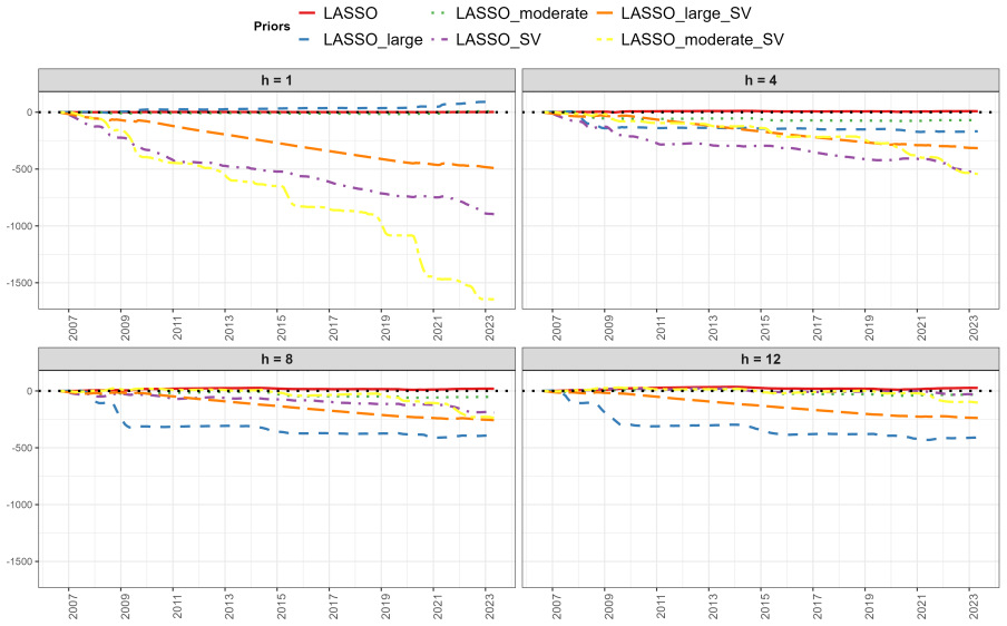
On its own terms, the paper's discovery is an empirical regularity: in a direct multi-step forecasting exercise for Thai headline CPI, models without stochastic volatility dominate their SV-augmented counterparts, and the gap grows with the predictor set. The large 56-predictor Horseshoe, Horseshoe+, Dirichlet-Laplace, and Lasso regressions produce relative RMSE values well below 1 at the one-month horizon (for example 0.15–0.16 for HS and HS+, 0.21 for DL) and relative tail-weighted CRPS values around 0.58–0.62, while the SV versions, especially HS with SV, show severely negative cumulative log predictive likelihoods. The paper also reports an asymmetry: left-tail (deflationary) risk is captured well by the heavy-tailed shrinkage priors, whereas right-tail (inflationary-spike) forecasting is unstable, with some priors breaking down under stress. Finally, the Horseshoe's shrinkage factor $\kappa$ identifies a small set of supply-side CPI components plus the number of alien work permits in Bangkok as the predictors that consistently resist shrinkage, which the authors read as the cost-push signature of a credible inflation-targeting regime.
Load-bearing premise
The head-to-head that supports the title claim assumes the SV-augmented models and the Dirichlet-Laplace prior are implemented correctly, but the paper gives no equations, likelihood, or sampler details for the SV versions and never defines the Dirichlet-Laplace prior, so the reported rankings cannot be audited or reproduced.
Editorial extensions
If this is right
- Policymakers at the Bank of Thailand can treat the 56-predictor Horseshoe, Dirichlet-Laplace, or Lasso regression without SV as a better short-run inflation forecast than SV-augmented alternatives, especially at the one-month horizon.
- In high-dimensional settings, adding stochastic volatility is predicted to reduce rather than improve forecast accuracy, so model builders should decide on the predictor set before adding SV.
- Persistent high-$\kappa$ variables such as Eggs & Dairy, Electricity/Fuel/Water, and Bangkok alien work permits give a short list of supply-side indicators to watch for cost-push inflation under the targeting regime.
- Left-tail deflationary forecasts are more trustworthy than right-tail inflationary-surge forecasts, so tail-risk reporting should report left and right quantile scores separately rather than one average.
- The COVID-19 sub-period results suggest the no-SV large models also hold up in crisis episodes, implying the finding is not limited to calm periods.
Reading between the lines
- If the result holds beyond Thailand, it suggests that for small open inflation-targeting economies with relatively stable volatility, the default assumption that SV improves density forecasts should be reversed; a testable extension is to rerun the same direct-forecast design on Indonesia, the Philippines, or other emerging economies.
- The right-tail weakness may be partly an artifact of the chosen quantile weights; a natural test is to tilt qwCRPS weights even more heavily toward the upper 5% quantile and see whether the large shrinkage priors recover their rank or whether the failure is intrinsic.
- The Horseshoe-$\kappa$ ranking could be turned into a real-time monitoring dashboard: tracking whether supply-side CPI components move above $\kappa = 0.6$ would give a data-driven early signal of cost-push pressure before inflation materializes.
- Because the SV implementations are not specified in the paper, a task for future work is to re-estimate with a standard SV likelihood, such as an AR(2) mean equation with a log-volatility random walk, and check whether the ordering is an artifact of estimation noise rather than a property of SV itself.
Signed reviews
Editorial analysis
A structured set of objections, weighed in public.
Referee Report
Summary. The paper compares Bayesian shrinkage priors (noninformative, Ridge, Adaptive Lasso, Spike-and-Slab, Horseshoe, Horseshoe+, and Dirichlet–Laplace) for univariate out-of-sample forecasting of Thai CPI inflation. Forecasts are produced at horizons h = 1, 4, 8, 12 in three predictor settings (AR(2) only, moderate with 20 predictors, large with 56 predictors), evaluated by relative RMSE, quantile-weighted CRPS (uniform, tails, right, left), and cumulative log predictive likelihood. The authors compare these models with and without stochastic volatility and conclude that SV-augmented models underperform non-SV counterparts, that HS, DL and LASSO in the large predictor setting are superior across multiple horizons, and that left-tail (deflationary) risks are better captured than right-tail (inflationary) risks. A final section interprets Horseshoe shrinkage weights (kappa) as identifying supply-side drivers of Thai inflation.
Significance. If the empirical claims were fully supported, the paper would provide a useful case study of high-dimensional univariate Bayesian forecasting for an emerging economy, and a cautionary note on the value of stochastic volatility in this context. The design has components that are appropriate for this purpose: a monthly Thai dataset with a broad set of predictors, a rolling-window out-of-sample scheme, multiple forecast horizons, and a range of proper scoring rules. The paper also engages with an interesting substantive question about sparse versus dense predictor sets and tail risks in inflation. However, in its current form the significance cannot be assessed because the central results are internally inconsistent and key model components are never specified. The paper does not ship reproducible code or data, and several numerical claims in the text do not match the tables.
major comments (5)
- [Section 2] The Dirichlet–Laplace (DL) prior, which appears in the abstract, in all results tables (Tables 2–5), and in the conclusions, is never defined. Section 2 defines the noninformative, Ridge, Adaptive Lasso, Spike-and-Slab, Horseshoe, and Horseshoe+ priors (Eqs. 4–11), but DL is absent from the methodology. Without the prior distribution, its hyperparameters, the likelihood, or the sampling algorithm, the DL results cannot be audited or reproduced. This is load-bearing because the abstract's headline claim ('HS, DL and LASSO in large-sized model setting without SV exhibit superior performance') directly depends on a model that is never specified.
- [Section 5, Figures 1–3] The SV-augmented models ('HS SV', 'RIDGE SV', 'LASSO SV', and their moderate and large versions) are not specified. The text refers to Stock and Watson (2007) but gives no state equation, no prior distribution for the volatility parameters, no estimation algorithm, and no convergence diagnostics for the SV extensions of the Bayesian regression in Eq. (1). The central conclusion that SV 'appears to increase estimation noise rather than improving forecast accuracy' rests entirely on these undefined implementations. As presented, the comparison between SV and non-SV models cannot be audited or reproduced, and the possibility of a mis-specified or incorrectly estimated SV model cannot be ruled out.
- [Table 2 and Abstract/Conclusion] The abstract and conclusion claim that LASSO in the large-sized model without SV exhibits superior performance across multiple horizons, but Table 2 contradicts this. For the full period, LASSO large has relative RMSE 1.05 at h=4, 1.54 at h=8, and 2.69 at h=12, all worse than the benchmark; in the pandemic period, the relative RMSE is 1.08 at h=4 and 1.77 at h=12. Section 4 itself states that LASSO shows 'substantial degradation at h=8 and h=12'. The conclusion statement that 'the LASSO large model without SV consistently provides superior performance across both short- and long-term horizons' is therefore inconsistent with the reported results, and this inconsistency affects the main policy message of the paper.
- [Section 5, LPL numbers] The cumulative log predictive likelihood (LPL) values in Section 5 (e.g., HS 1.6045 vs. HS SV -1070.0754 at h=1; HS moderate 35.2046 vs. HS moderate SV -1549.2438 at h=4; HS large -6.0832 vs. HS large SV -1116.3535 at h=12) are not defined and appear implausible. No formula for cumulative LPL is given, no table reports these values, and no explanation is provided for the order of magnitude. A value of -1070 for a cumulative monthly log score over roughly 40 evaluation periods would imply an average log likelihood near -26, which is not credible for a well-calibrated predictive density. These numbers are the primary evidence for the SV-versus-non-SV conclusion, but as they stand they suggest a computational failure or a scoring convention that is not described, rather than a reliable empirical result.
- [Section 4.1] Several prose numbers in Section 4.1 do not appear in the tables. The text claims 'Ridge ... an extreme qwCRPS score of almost 200%', but Table 3 (tails) reports RIDGE large full h=1 = 1.03, not approximately 2. The text claims 'DL suffered a catastrophic breakdown (7.65)' in the right-weighted CRPS discussion, but Table 4 (right) shows DL large h=4 = 0.93 (full) and 0.80 (pandemic), and no value near 7.65 appears in any table. The same section refers to DL 'extreme inefficiencies (6.51 in full range, 3.50 in pandemic)', which also do not appear in Tables 3–5. These discrepancies mean the density-forecast results, which support the tail-risk asymmetry claim, cannot be reliably interpreted from the manuscript as written.
minor comments (6)
- [Section 2, introductory paragraph] The text says 'we investigate the forecasting performance of six priors' but then lists noninformative, Ridge, Lasso, Horseshoe, Horseshoe+, and Spike-and-Slab plus, later, DL in the results; the count and the list should be reconciled. Also, the intro sentence about frequentist approaches is an incomplete fragment.
- [Equation (6)] The Adaptive Lasso notation is confusing: lambda is used as the Laplace rate on the left-hand side and as the local regularization parameter on the right-hand side, and the 'epsilon' in the denominator is undefined. Clarifying these definitions would help reproducibility.
- [Section 6] The driver narrative in Section 6 interprets the Horseshoe shrinkage weight kappa from the in-sample full-period fit as evidence of causal importance for Thai inflation. This is not supported by an out-of-sample validation or a formal test, and the reader should be told that these are descriptive posterior summaries rather than identified causal effects. This is not central to the forecasting comparison, but it is presented as a substantive finding.
- [Section 5, Ridge discussion] The sentence 'In my opinion, the results highlight an important trade-off...' uses a first-person phrase that is unusual in a co-authored research paper and should be reworded.
- [Table 6 / Section 4] The data description says 'the first 20 series are included in moderate-sized model setup', but the list in Table 6 includes 56 series and the first series is CPI; it is unclear whether the moderate model includes CPI plus 19 predictors or 20 predictors including CPI. Please clarify the exact variable sets.
- [Throughout] Several references and terms have typographical issues (e.g., 'Hern' andez-Lobato' with a stray space, 'Ba' nbura', 'sucha as', 'a the AR(2)'). A careful proofread would be needed before resubmission. The paper also does not state whether data and code are available for reproducibility.
Circularity Check
No circularity: the forecast comparison is an out-of-sample empirical exercise; missing model definitions are an auditability flaw, not a circular step.
full rationale
The paper's central claims are empirical rankings of Bayesian shrinkage priors for Thai inflation, evaluated by out-of-sample RMSE, qwCRPS, and LPL. The benchmark is a noninformative-prior AR(2) model defined in Eq. (4), and each prior is fitted and then evaluated on rolling holdout windows. No forecast quantity is constructed from a fitted value of the same target, and no 'prediction' is a re-labelled fit. The SV-versus-non-SV comparison in Section 5 uses cumulative log predictive likelihood from separate model fits; although the SV-augmented models and the DL prior are never formally specified, that omission is a reproducibility and correctness problem, not circularity. Section 6's driver narrative uses posterior shrinkage coefficients (kappa) from the Horseshoe fit to describe which predictors resist shrinkage; this is interpretive and does not feed back into the forecast evaluation or the headline rankings. The abstract's statement that LASSO large performs well without SV is contradicted by Table 2, but an internal inconsistency is not circularity. Self-citations such as Hossain and Arwatchanakarn (2016) are background references and are not load-bearing for the forecast results. No equation-level recycling, no fitted-input-called-prediction, and no uniqueness theorem imported from the authors' prior work were found. The derivation chain is self-contained with respect to the forecast comparisons, so the circularity score is 0.
Assumptions & free parameters
free parameters (7)
- c (variance scale of noninformative prior) =
10^4
- Ridge global shrinkage lambda =
not reported
- Adaptive Lasso adaptiveness exponent gamma =
not reported
- Adaptive Lasso numerical stability epsilon =
not reported
- Spike-and-Slab hyperparameters (a, b, alpha, beta) =
not reported
- Rolling window length =
128 observations
- Predictor set sizes =
20 (moderate), 56 (large)
assumptions (5)
- domain assumption The linear Gaussian likelihood y ~ N(X*beta, sigma^2 I) adequately describes Thai inflation.
- domain assumption YoY growth transformation makes all 56 series stationary.
- ad hoc to paper The UC-SV and SV-augmented models follow Stock and Watson (2007) and are correctly estimated.
- ad hoc to paper The Horseshoe posterior shrinkage weight kappa indicates causal importance for inflation.
- domain assumption Direct multi-step forecasting with a rolling 128-observation window gives comparable predictive densities across horizons.
Cite this review
Pith. "Pith review of Forecasting Thai inflation from univariate Bayesian regression perspective." pith.science (2026). https://pith.science/paper/BJ7OPR76
@misc{pith2026250505334,
  author       = {Pith},
  title        = {Pith review of: Forecasting Thai inflation from univariate Bayesian regression perspective},
  year         = {2026},
  howpublished = {\url{https://pith.science/paper/BJ7OPR76}},
  note         = {Machine review of arXiv:2505.05334}
}
read the original abstract
This study investigates the forecasting performance of Bayesian shrinkage priors in predicting Thai inflation in a univariate setup, with a particular interest in comparing those more advance shrinkage prior to a likelihood dominated/noninformative prior. Our forecasting exercises are evaluated using Root Mean Squared Error (RMSE), Quantile-Weighted Continuous Ranked Probability Scores (qwCRPS), and Log Predictive Likelihood (LPL). The empirical results reveal several interesting findings: SV-augmented models consistently underperform compared to their non-SV counterparts, particularly in large predictor settings. Notably, HS, DL and LASSO in large-sized model setting without SV exhibit superior performance across multiple horizons. This indicates that a broader range of predictors captures economic dynamics more effectively than modeling time-varying volatility. Furthermore, while left-tail risks (deflationary pressures) are well-controlled by advanced priors (HS, HS+, and DL), right-tail risks (inflationary surges) remain challenging to forecast accurately. The results underscore the trade-off between model complexity and forecast accuracy, with simpler models delivering more reliable predictions in both normal and crisis periods (e.g., the COVID-19 pandemic). This study contributes to the literature by highlighting the limitations of SV models in high-dimensional environments and advocating for a balanced approach that combines advanced shrinkage techniques with broad predictor coverage. These insights are crucial for policymakers and researchers aiming to enhance the precision of inflation forecasts in emerging economies.
Figures


Figures from the paper (4 more)


Reference graph
Works this paper leans on
-
[1]
Alp, M. H. and Elekdag, S. (2012). Shock Therapy! What Role for Thai Monetary Policy? International Monetary Fund
work page 2012
-
[2]
Ayales, E. (2002). 16 inflation targeting: Statistical issues suggested by the experience of six emerging market countries. Statistical Implications of Inflation Targeting
work page 2002
-
[3]
Bai, R., Ro c kov \'a , V., and George, E. I. (2021). Spike-and-slab meets lasso: A review of the spike-and-slab lasso. Handbook of Bayesian variable selection , pages 81--108
work page 2021
-
[4]
Ba \'n bura, M., Giannone, D., and Reichlin, L. (2010). Large bayesian vector auto regressions. Journal of applied Econometrics , 25(1):71--92
work page 2010
-
[5]
Bedoui, A. and Lazar, N. A. (2020). Bayesian empirical likelihood for ridge and lasso regressions. Computational Statistics & Data Analysis , 145:106917
work page 2020
-
[6]
Bhadra, A., Datta, J., Polson, N. G., and Willard, B. (2017). The horseshoe+ estimator of ultra-sparse signals
work page 2017
-
[7]
Bhadra, A., Datta, J., Polson, N. G., and Willard, B. (2019). Lasso meets horseshoe. Statistical Science , 34(3):405--427
work page 2019
-
[8]
S., and Dunson, D
Bhattacharya, A., Pati, D., Pillai, N. S., and Dunson, D. B. (2015). Dirichlet--laplace priors for optimal shrinkage. Journal of the American Statistical Association , 110(512):1479--1490
2015
Show all 54 references
-
[9]
and Rukumnuaykit, P
Bryant, J. and Rukumnuaykit, P. (2007). Does immigration to thailand reduce the wages of thai workers. Institute for Population and Social Research (IPSR), Mahidol University. Mimeo
2007
-
[10]
E., and Marcellino, M
Carriero, A., Clark, T. E., and Marcellino, M. G. (2020). Nowcasting tail risks to economic activity with many indicators
2020
-
[11]
M., Polson, N
Carvalho, C. M., Polson, N. G., and Scott, J. G. (2010). The horseshoe estimator for sparse signals. Biometrika , 97(2):465--480
2010
-
[12]
Chevillon, G. (2007). Direct multi-step estimation and forecasting. Journal of Economic Surveys , 21(4):746--785
2007
-
[13]
Clark, T. E. (2011). Real-time density forecasts from bayesian vector autoregressions with stochastic volatility. Journal of Business & Economic Statistics , 29(3):327--341
2011
-
[14]
E., Huber, F., Koop, G., and Marcellino, M
Clark, T. E., Huber, F., Koop, G., and Marcellino, M. (2024). Forecasting us inflation using bayesian nonparametric models. The Annals of Applied Statistics , 18(2):1421--1444
2024
-
[15]
E., Huber, F., Koop, G., Marcellino, M., and Pfarrhofer, M
Clark, T. E., Huber, F., Koop, G., Marcellino, M., and Pfarrhofer, M. (2021). Tail forecasting with multivariate bayesian additive regression trees
2021
-
[16]
and Hendry, D
Clements, M. and Hendry, D. F. (1998). Forecasting economic time series . Cambridge University Press
1998
-
[17]
L., Hou, C., and Poon, A
Cross, J. L., Hou, C., and Poon, A. (2019). Macroeconomic forecasting with large bayesian vars: Global-local priors and the illusion of sparsity. International Journal of Forecasting
2019
-
[18]
Direkudomsak, W. (2016). Inflation dynamics and inflation expectations in thailand. BIS Paper , (89y)
2016
-
[19]
George, E. I. and McCulloch, R. E. (1993). Variable selection via gibbs sampling. Journal of the American Statistical Association , 88(423):881--889
1993
-
[20]
Giannone, D., Lenza, M., and Primiceri, G. E. (2015). Prior selection for vector autoregressions. Review of Economics and Statistics , 97(2):436--451
2015
-
[21]
Gneiting, T., Balabdaoui, F., and Raftery, A. E. (2007). Probabilistic forecasts, calibration and sharpness. Journal of the Royal Statistical Society: Series B (Statistical Methodology) , 69(2):243--268
2007
-
[22]
and Raftery, A
Gneiting, T. and Raftery, A. E. (2007). Strictly proper scoring rules, prediction, and estimation. Journal of the American Statistical Association , 102(477):359--378
2007
-
[23]
and Ranjan, R
Gneiting, T. and Ranjan, R. (2011). Comparing density forecasts using threshold-and quantile-weighted scoring rules. Journal of Business & Economic Statistics , 29(3):411--422
2011
-
[24]
and Amatyakul, P
Gongsiang, M. and Amatyakul, P. (2021). Inflation at risk in thailand. Technical report, Puey Ungphakorn Institute for Economic Research
2021
-
[25]
Hauzenberger, N., Huber, F., Marcellino, M., and Petz, N. (2021). Gaussian process vector autoregressions and macroeconomic uncertainty. arXiv preprint arXiv:2112.01995
2021 arXiv
-
[26]
M., and Dupont, P
Hern \'a ndez-Lobato, D., Hern \'a ndez-Lobato, J. M., and Dupont, P. (2013). Generalized spike-and-slab priors for bayesian group feature selection using expectation propagation. Journal of Machine Learning Research , 14(7)
2013
-
[27]
Hoerl, A. E. and Kennard, R. W. (1970). Ridge regression: Biased estimation for nonorthogonal problems. Technometrics , 12(1):55--67
1970
-
[28]
Hossain, A. A. and Arwatchanakarn, P. (2016). Inflation and inflation volatility in thailand. Applied Economics , 48(30):2792--2806
2016
-
[29]
Hossain, A. A. and Raghavan, M. (2020). The time-variant sources of inflation and inflation volatility and their interrelations and effects on macroeconomic fluctuations: Evidence from indonesia and thailand. Journal of Business and Economic Analysis , 3(03):228--267
2020
-
[30]
Huber, F., Koop, G., Onorante, L., Pfarrhofer, M., and Schreiner, J. (2020). Nowcasting in a pandemic using non-parametric mixed frequency vars. arXiv preprint arXiv:2008.12706
2020 arXiv
-
[31]
and Rao, J
Ishwaran, H. and Rao, J. S. (2005). Spike and slab gene selection for multigroup microarray data. Journal of the American Statistical Association , 100(471):764--780
2005
-
[32]
S., et al
Ishwaran, H., Rao, J. S., et al. (2005). Spike and slab variable selection: frequentist and bayesian strategies. The Annals of Statistics , 33(2):730--773
2005
-
[33]
S., Mitchell, J., and Vahey, S
Jore, A. S., Mitchell, J., and Vahey, S. P. (2010). Combining forecast densities from vars with uncertain instabilities. Journal of Applied Econometrics , 25(4):621--634
2010
-
[34]
Koirala, N. P. and Nyiwul, L. (2023). Inflation volatility: A bayesian approach. Research in Economics , 77(1):185--201
2023
-
[35]
Koop, G. (2010). Bayesian multivariate time series methods for empirical macroeconomics
2010
-
[36]
and Korobilis, D
Koop, G. and Korobilis, D. (2014). A new index of financial conditions. European Economic Review , 71:101--116
2014
-
[37]
Koop, G. M. (2003). Bayesian econometrics . John Wiley & Sons Inc
2003
-
[38]
Leng, C., Tran, M.-N., and Nott, D. (2014). Bayesian adaptive lasso. Annals of the Institute of Statistical Mathematics , 66:221--244
2014
-
[39]
and Primiceri, G
Lenza, M. and Primiceri, G. E. (2020). How to estimate a var after march 2020. Technical report, National Bureau of Economic Research
2020
-
[40]
Litterman, R. B. (1986). Forecasting with bayesian vector autoregressions—five years of experience. Journal of Business & Economic Statistics , 4(1):25--38
1986
-
[41]
and Wongpunya, N
Luangaram, P. and Wongpunya, N. (2022). Exploring the role of exchange rates in inflation targeting: Evidence from thailand. Available at SSRN 4269032
2022
-
[42]
and Schmidt, D
Makalic, E. and Schmidt, D. F. (2015). A simple sampler for the horseshoe estimator. IEEE Signal Processing Letters , 23(1):179--182
2015
-
[43]
Manopimoke, P. (2018). Thai inflation dynamics in a globalized economy. Journal of the Asia Pacific Economy , 23(3):465--495
2018
-
[44]
and Limjaroenrat, V
Manopimoke, P. and Limjaroenrat, V. (2017). Trend inflation estimates for thailand from disaggregated data. Economic Modelling , 65:75--94
2017
-
[45]
H., and Watson, M
Marcellino, M., Stock, J. H., and Watson, M. W. (2006). A comparison of direct and iterated multistep ar methods for forecasting macroeconomic time series. Journal of econometrics , 135(1-2):499--526
2006
-
[46]
McCracken, M. W. and McGillicuddy, J. T. (2019). An empirical investigation of direct and iterated multistep conditional forecasts. Journal of Applied Econometrics , 34(2):181--204
2019
-
[47]
Mitchell, T. J. and Beauchamp, J. J. (1988). Bayesian variable selection in linear regression. Journal of the american statistical association , 83(404):1023--1032
1988
-
[48]
and Casella, G
Park, T. and Casella, G. (2008). The bayesian lasso. Journal of the american statistical association , 103(482):681--686
2008
-
[49]
G., Scott, J
Polson, N. G., Scott, J. G., and Windle, J. (2014). The bayesian bridge. Journal of the Royal Statistical Society Series B: Statistical Methodology , 76(4):713--733
2014
-
[50]
Stock, J. H. and Watson, M. W. (2002). Macroeconomic forecasting using diffusion indexes. Journal of Business & Economic Statistics , 20(2):147--162
2002
-
[51]
Stock, J. H. and Watson, M. W. (2007). Why has us inflation become harder to forecast? Journal of Money, Credit and banking , 39:3--33
2007
-
[52]
B., Hyndman, R
Taieb, S. B., Hyndman, R. J., et al. (2012). Recursive and direct multi-step forecasting: the best of both worlds , volume 19. Department of Econometrics and Business Statistics, Monash Univ
2012
-
[53]
Tibshirani, R. (1996). Regression shrinkage and selection via the lasso. Journal of the Royal Statistical Society Series B: Statistical Methodology , 58(1):267--288
1996
-
[54]
Zou, H. (2006). The adaptive lasso and its oracle properties. Journal of the American statistical association , 101(476):1418--1429
2006
Reviewed August 15, 2026 · model on record in the stance chip above.
Discussion (0). Continue with ORCID to comment.