REVIEW 3 major objections 6 minor 51 references
Testing thermal conductivity models with equilibrium molecular dynamics simulations of the one component plasma
T0 review · 3 major / 6 minor · reviewed 2026-08-14 · deepseek-v4-flash
Pith's one-line read New simulations give accurate one-component plasma conductivity, and no theory works at strong coupling.
desk verdict A valuable, mostly reliable OCP thermal conductivity benchmark that advances the field, but the unspecified production ensemble and overstated 2% accuracy claim need fixing before publication. read the letter →
The pith
A machine-rendered reading of the paper's core claim, the machinery that carries it, and where it could break.
The reading
What carries the argument
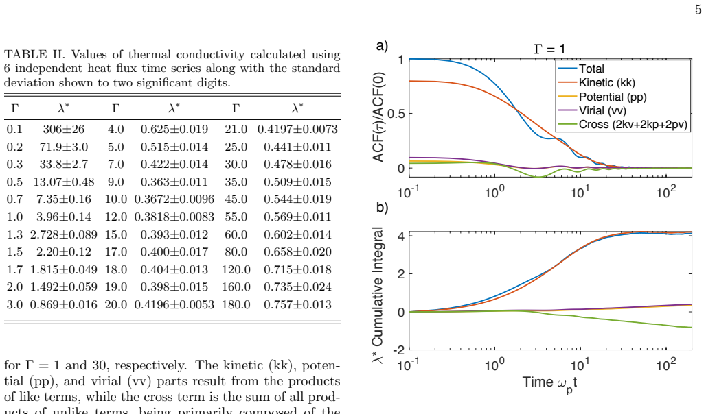
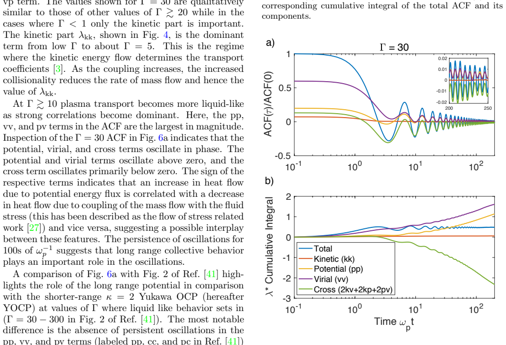
The machinery is the Green-Kubo relation with a component-resolved heat-flux autocorrelation. The heat flux $\mathbf{j}$ is split into a kinetic part (particle mass flow carrying kinetic energy), a potential part (potential energy transported by mass flow), and a virial part (stress coupled to mass flow). The paper computes the autocorrelation of each part and of the cross terms, showing for the first time in the OCP that at $\Gamma\gtrsim10$ the potential and virial terms oscillate in phase and dominate the transport. A second piece of machinery is the noise-control protocol: because the ACF tail obeys the $1/\tau$ noise scaling of Zwanzig-Ailawadi, the authors use $6\times10^5\,\omega_p^{-1}$ time series and average the cumulative integral over a window where oscillations have decayed but noise has not yet built up.
What would settle it
Re-run the Γ = 30 simulation with the thermostat explicitly disabled during production and compare the heat-flux autocorrelation and integrated conductivity with the reported value; if the conductivity shifts by more than the stated error bars, the dataset is biased. Alternatively, an independent non-equilibrium MD calculation at Γ = 30 that reproduces the reported λ* would support the claim, while disagreement would falsify it.
Extended reading notes
Core claim
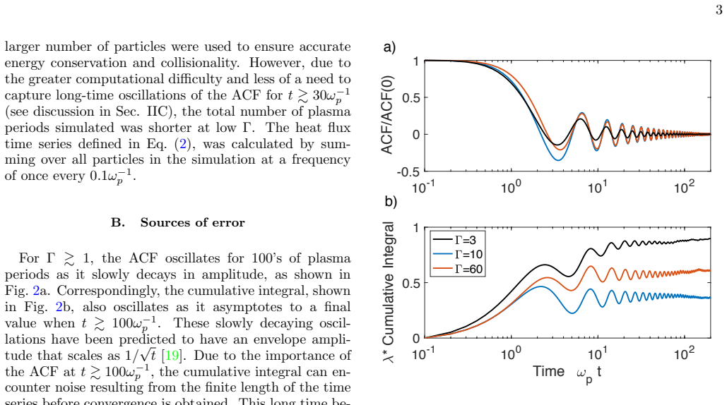
The central discovery is that the OCP heat-flux autocorrelation function (ACF) has a slowly decaying oscillatory envelope, predicted to scale as $1/\sqrt{t}$, so the cumulative Green-Kubo integral is still oscillating by about 5% at $t=100\,\omega_p^{-1}$ and only converges after hundreds of plasma periods. Prior equilibrium MD runs of roughly $400$ and $8000\,\omega_p^{-1}$ were too short, which explains the discrepancies with non-equilibrium MD. The authors run $6\times10^5\,\omega_p^{-1}$ trajectories, verify noise levels against cross-correlations of different heat-flux components, and average the cumulative integral over $[100,150]\,\omega_p^{-1}$. The resulting dimensionless conductivity $\lambda^*=\lambda/(n\omega_p k_B a^2)$ agrees with non-equilibrium data for $\Gamma\ge2$ and extends down to $\Gamma=0.1$. Decomposing the heat flux into kinetic, potential, and virial parts shows that the kinetic term dominates up to $\Gamma\approx5$, while for $\Gamma\gtrsim10$ the potential, virial, and their cross term are largest; no theory that treats only kinetic transport can capture this regime.
Load-bearing premise
The paper never states whether the Nose-Hoover thermostat used during equilibration is turned off during the production runs; if the thermostat remains coupled, it could damp the heat-flux autocorrelation and bias all reported conductivities.
Editorial extensions
If this is right
- The new dataset interpolates from weak coupling to solidification at $\Gamma\approx170$ and provides a fitted formula (Eqs. 7–9) for use in hydrodynamic simulations of dense plasmas.
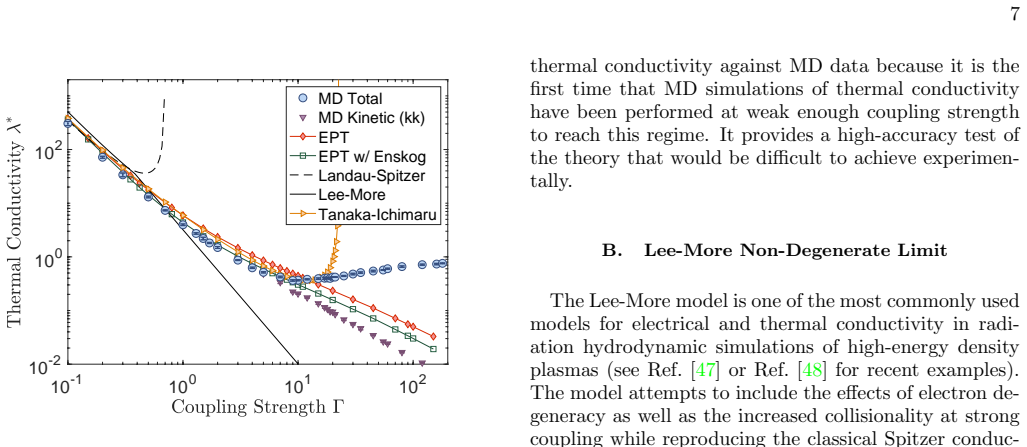
- Landau-Spitzer theory is confirmed only for $\Gamma\lesssim0.3$; using it beyond that coupling overestimates the thermal conductivity.
- The Lee-More model's ad hoc replacement of the Debye length by the ion-sphere radius is shown to be inadequate for $\Gamma\gtrsim1$, a relevant caveat for high-energy-density simulations that use this model.
- Existing theories such as EPT can describe the kinetic component of the heat flux to fairly strong coupling, but none describes the potential-virial dominated regime, indicating a need for transport theories that include multi-particle dynamics.
- The component decomposition reveals that at $\Gamma\approx9$ the conductivity reaches a minimum where the kinetic term becomes smaller than the sum of potential and virial terms, providing a benchmark for future theories.
Reading between the lines
- The in-phase oscillations of the potential and virial ACF components and the opposite-signed cross term suggest that a conserved quantity, such as an enthalpy current, may be exchanged between the two channels; a mode-coupling or hydrodynamic description might reproduce this cancellation and extend theory past $\Gamma\approx10$.
- The $1/\sqrt{t}$ noise envelope implies that even longer runs, or variance-reduction estimators such as cepstral analysis, could push the accuracy below 2% and extend the dataset to lower $\Gamma$ or to two-component plasmas without prohibitive cost.
- A direct test of the unstated thermostat protocol, whether the Nose-Hoover thermostat is removed during production, would determine whether the reported conductivities are biased; this check is not addressed in the paper but is a necessary reproducibility test.
- The different ranges of validity of EPT for diffusion, shear viscosity, and thermal conductivity suggest that each transport coefficient has a different sensitivity to many-body correlations, which could guide which coefficient is best for benchmarking new strong-coupling theories.
Signed reviews
Editorial analysis
A structured set of objections, weighed in public.
Referee Report
Summary. The manuscript reports equilibrium molecular dynamics (MD) simulations of the thermal conductivity of the one-component plasma (OCP) using the Green-Kubo formalism, covering Γ from 0.1 to 180. The authors use long heat-flux time series (up to 6×10^5 ω_p^{-1}), analyze statistical noise via cross-correlations and the Zwanzig-Ailawadi estimate, decompose the conductivity into kinetic, potential, virial, and cross contributions, and compare the total conductivity against Landau-Spitzer, Lee-More, Tanaka-Ichimaru, and Effective Potential Theory (EPT). They conclude that Landau-Spitzer agrees with simulations for Γ≲0.3, that EPT and Tanaka-Ichimaru are accurate up to Γ≈7, and that none of the models captures the regime Γ≳10, where potential and virial heat-flux components dominate. The paper also provides analytic fits to the MD data.
Significance. If the reported data are reliable, this is a valuable benchmark: it is the first equilibrium MD dataset extending to Γ<1, provides the first MD test of Landau-Spitzer thermal conductivity, and quantitatively documents the failure of binary-collision-based theories at strong coupling. The component decomposition (kinetic/potential/virial) is a useful diagnostic for future theory development. The error analysis is thoughtful, using six independent time series, cross-correlation noise estimators, and explicit comparison with the predicted 1/τ scaling. The agreement with prior non-equilibrium MD for Γ≥2 partially mitigates concerns about the equilibrium method. However, the central claim of 'accurate data' is weakened by an unspecified production-phase ensemble and by an accuracy statement that is not consistent with the tabulated statistical uncertainties.
major comments (3)
- [Sec. IIA, Eq. (1)] The manuscript specifies a Nosé-Hoover thermostat only for the equilibration phase and never states whether the thermostat is turned off during the production runs. Because the Green-Kubo relation in Eq. (1) is derived for Hamiltonian dynamics, and because the paper itself emphasizes heat-flux autocorrelation oscillations persisting for hundreds of ω_p^{-1} at Γ≥10, coupling a thermostat during production could damp those oscillations and bias the reported conductivities. The agreement with non-equilibrium MD in Fig. 1 for Γ≥2 is reassuring but does not validate the new Γ<0.5 data used for the Landau-Spitzer test. Please state explicitly the ensemble used during data collection (e.g., NVE or NVT) and, if NVT is used, justify its consistency with the Green-Kubo formula.
- [Abstract and Table II] The abstract's claim that 6×10^5 ω_p^{-1} time series allow '≲2% accuracy' is not supported by the Table II numbers if those are standard deviations of the six independent time series: the relative standard deviations at Γ=0.5, 1.0, 2.0, and 5.0 are about 3.7%, 3.5%, 4.0%, and 2.7%, respectively. If the tabulated values are instead standard errors of the mean (standard deviation divided by sqrt(6)), the text should say so explicitly and the abstract should state which quantity corresponds to 'accuracy.' Please reconcile the abstract with the tabulated uncertainties.
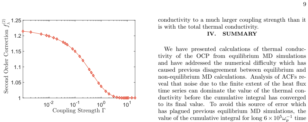
- [Sec. IIC] The choice of the averaging window [100,150] ω_p^{-1} for Γ≥0.5 is justified only by the qualitative statement that alternate windows do not change results 'significantly.' Since the cumulative integral still exhibits oscillations at the ~5% level at t=100 ω_p^{-1}, a quantitative sensitivity analysis (e.g., a table or figure showing λ* for several averaging windows) is needed to support the claimed accuracy. In addition, for Γ<0.5 a different saturation-based method is used; the crossover between methods and its effect on the reported values should be documented.
minor comments (6)
- [Sec. IIB, Eq. (4)] The notation ⟨...⟩ is used both for the ensemble average in Eq. (1) and for the finite-time average in Eq. (3); please distinguish the two, for example by using a subscript for the time-average.
- [Reference [41]] Reference [41] lists the first author as 'Z. Donk' instead of 'Z. Donkó' and omits the publication year; please correct the citation.
- [Sec. IIC, Table II] The table caption states 'standard deviation' but the text says the six values were 'averaged ... with their standard deviation.' Please specify whether the reported error is the standard deviation of the six values or the standard error of the mean, and use consistent terminology throughout.
- [Sec. IIIA and Eq. (11)] In the discussion of the Landau-Spitzer limit, the text says the kinetic fit is 'proportional to C/ln(DΓ^{-3/2})' at low Γ, but the full expression in Eq. (7) also contains the prefactor Γ^{-5/2}; please correct this limiting-form description.
- [Sec. IIC] The word 'neagitive' appears in the sentence 'reaches its maximum neagitive value'; this should be 'negative.'
- [Sec. IIC, Eq. (9)] The text states that the fit of Eq. (9) passes through all markers 'with one exception'; please identify which data point is the exception, since this is not otherwise evident from Fig. 4.
Circularity Check
No significant circularity: the MD data are independent measurements, the tested models are not fitted to these data, and the paper's own fits are explicitly labeled as fits.
full rationale
The central derivation chain is: run equilibrium MD, compute the Green-Kubo heat-flux ACF integral, and compare the resulting λ* with four theoretical models. None of the models is fitted to the new conductivity data. EPT (Refs. 21, 44) is the authors' own theory, but in this paper it is evaluated by computing g(r) from HNC closure and solving Chapman-Enskog collision integrals (Eqs. 17-21); the text reports that EPT fails for Γ ≳ 7 (Fig. 7), which shows the theory is not used to define the outcome. Tanaka-Ichimaru uses a bridge function fitted to OCP MD static structure (Sec. III.C), but that is a static pair-correlation input, not the transport coefficient being predicted. The fits in Eqs. (7)-(9) are introduced for convenience and explicitly called 'fit' (Sec. IIC), so they are not disguised predictions. The Landau-Spitzer test uses the new independent low-Γ MD data. Self-citations (Refs. 4, 7, 21, 44, 46, 52) are theoretical derivations or prior comparisons of other transport coefficients; none incorporates the thermal conductivity values reported here. The only notable manuscript omission—the absence of an explicit statement whether the Nosé-Hoover thermostat is removed during production—is a reproducibility/algorithmic concern, not a circularity, and per the hard rules no circularity score is assigned to it.
Assumptions & free parameters
free parameters (5)
- C (λ_kk fit, Eq. 7) =
3.766
- D (λ_kk fit, Eq. 7) =
1.52
- Padé coefficients p_i, q_i for λ_kk (Eq. 7) =
Table III
- Padé coefficients p_i, q_i for λ_pp,pv,vv (Eq. 8) =
Table III
- Biexponential coefficients p_i for λ_kv,kp (Eq. 9) =
Table III
assumptions (6)
- standard math Green-Kubo relation (Eq. 1) correctly gives thermal conductivity from the equilibrium heat flux ACF.
- domain assumption The OCP model (Coulomb potential in a uniform neutralizing background) is the relevant reference system for strongly coupled plasmas.
- domain assumption The production phase of the MD is in the correct equilibrium ensemble (thermostat-free NVE or equivalent) so that j(t) fluctuations are unperturbed by the thermostat.
- domain assumption The heat flux ACF has converged by t=150ω_p^{-1}, so the [100,150] averaging window yields the true Green-Kubo integral.
- domain assumption For the Tanaka-Ichimaru model, the bridge function b(r) is taken from fits to OCP MD pair distributions (Ref. 20); for EPT, the HNC closure (Eqs. 15-16) provides adequate g(r).
- domain assumption PPPM with a 50^3 mesh and 5a cutoff accurately represents the bare Coulomb interaction in the OCP.
Cite this review
Pith. "Pith review of Testing thermal conductivity models with equilibrium molecular dynamics simulations of the one component plasma." pith.science (2026). https://pith.science/paper/BS3U3JXS
@misc{pith2026190808415,
  author       = {Pith},
  title        = {Pith review of: Testing thermal conductivity models with equilibrium molecular dynamics simulations of the one component plasma},
  year         = {2026},
  howpublished = {\url{https://pith.science/paper/BS3U3JXS}},
  note         = {Machine review of arXiv:1908.08415}
}
abstract
Equilibrium molecular dynamics simulations are used to calculate the thermal conductivity of the one component plasma (OCP) via the Green-Kubo formalism over a broad range of Coulomb coupling strength, $0.1\le\Gamma\le180$. These simulations address previous discrepancies between computations using equilibrium versus nonequilibrium methods. Analysis of heat flux autocorrelation functions show that very long ($6\times10^5\omega_p^{-1}$) time series are needed to reduce the noise level to allow $\lesssim2\%$ accuracy. The new simulations provide the first accurate data for $\Gamma \lesssim 1$. This enables a test of the traditional Landau-Spitzer theory, which is found to agree with the simulations for $\Gamma \lesssim 0.3$. It also enables tests of theories to address moderate and strong Coulomb coupling. Two are found to provide accurate extensions to the moderate coupling regime of $\Gamma \lesssim 10$, but none are accurate in the $\Gamma \gtrsim 10$ regime where potential energy transport and coupling between mass flow and stress dominate thermal conduction.
Figures


Figures from the paper (5 more)

Reference graph
Works this paper leans on
-
[1]
M. Baus and J.-P. Hansen, Phys. Rep. 59, 1 (1980). [2] S. Chapman and T. G. Cowling, Cambridge: University Press, 1970, 3rd ed. (1970). 10
work page 1980
-
[3]
J. Ferziger and H. Kaper, Mathematical Theory of Trans- port Processes in Gases (North-Holland Publishing Com- pany, 1972)
work page 1972
- [4]
-
[5]
J. P. Hansen, I. R. McDonald, and E. L. Pollock, Phys. Rev. A 11, 1025 (1975)
work page 1975
- [6]
-
[7]
Accurate Determination of the Shear Viscosity of the One-Component Plasma
J. Daligault, K. Ø. Rasmussen, and S. D. Baal- rud, Phys. Rev. E 90, 033105 (2014), arXiv:1407.3875 [physics.plasm-ph]
work page Pith review arXiv 2014
- [8]
-
[9]
Z. Donk´ o, B. Ny´ ıri, L. Szalai, and S. Holl´ o, Phys. Rev. Lett. 81, 1622 (1998)
work page 1998
Show all 51 references
-
[10]
Donk´ o and P
Z. Donk´ o and P. Hartmann, Phys. Rev. E 69, 016405 (2004)
2004
-
[11]
E. L. Vold, R. M. Rauenzahn, C. H. Aldrich, K. Molvig, A. N. Simakov, and B. M. Haines, Physics of Plasmas 24, 042702 (2017)
2017
-
[12]
S. X. Hu, V. N. Goncharov, P. B. Radha, S. P. Regan, and E. M. Campbell, Nuclear Fusion 59, 032011 (2019)
2019
-
[13]
S. X. Hu, L. A. Collins, T. R. Boehly, Y. H. Ding, P. B. Radha, V. N. Goncharov, V. V. Karasiev, G. W. Collins, S. P. Regan, and E. M. Campbell, Physics of Plasmas 25, 056306 (2018)
2018
-
[14]
S. X. Hu, L. A. Collins, T. R. Boehly, J. D. Kress, V. N. Goncharov, and S. Skupsky, Phys. Rev. E 89, 043105 (2014)
2014
-
[15]
A. I. Chugunov and P. Haensel, Monthly No- tices of the Royal Astronomical Society 381, 1143 (2007), http://oup.prod.sis.lan/mnras/article- pdf/381/3/1143/3654270/mnras0381-1143.pdf
2007
-
[16]
Nunomura, D
S. Nunomura, D. Samsonov, S. Zhdanov, and G. Morfill, Phys. Rev. Lett. 95, 025003 (2005)
2005
-
[17]
Bannasch, J
G. Bannasch, J. Castro, P. McQuillen, T. Pohl, and T. C. Killian, Phys. Rev. Lett. 109, 185008 (2012)
2012
-
[18]
T. S. Strickler, T. K. Langin, P. McQuillen, J. Daligault, and T. C. Killian, Phys. Rev. X 6, 021021 (2016)
2016
-
[19]
M. C. Marchetti and T. R. Kirkpatrick, Phys. Rev. A 32, 2981 (1985)
1985
-
[20]
Tanaka and S
S. Tanaka and S. Ichimaru, Phys. Rev. A34, 4163 (1986)
1986
-
[21]
S. D. Baalrud and J. Daligault, Physical Review Letters 110, 235001 (2013), arXiv:1303.3202 [physics.plasm-ph]
2013 arXiv
-
[22]
Daligault, S
J. Daligault, S. D. Baalrud, C. E. Starrett, D. Saumon, and T. Sjostrom, Physical Review Letters 116, 075002 (2016)
2016
-
[23]
Bernu, P
B. Bernu, P. Vieillefosse, and J. P. Hansen, Physics Let- ters A 63, 301 (1977)
1977
-
[24]
Salin and J.-M
G. Salin and J.-M. Caillol, Physics of Plasmas 10, 1220 (2003)
2003
-
[25]
Donko and B
Z. Donko and B. Nyiri, Physics of Plasmas 7, 45 (2000), https://doi.org/10.1063/1.873824
2000 doi
-
[26]
Evans and G
D. Evans and G. Morriss, Statistical Mechanics of Nonequilibrium Liquids , DOAB Directory of Open Ac- cess Books (ANU E Press, 2007)
2007
-
[27]
Eu, Transport Coefficients of Fluids , Springer Series in Chemical Physics (Springer Berlin Heidelberg, 2010)
B. Eu, Transport Coefficients of Fluids , Springer Series in Chemical Physics (Springer Berlin Heidelberg, 2010)
2010
-
[28]
T. Ott, M. Bonitz, and Z. Donk´ o, Phys. Rev. E 92, 063105 (2015)
2015
-
[29]
Donk´ o, J
Z. Donk´ o, J. Goree, P. Hartmann, and B. Liu, Phys. Rev. E 79, 026401 (2009)
2009
-
[30]
Y. V. Khrustalyov and O. S. Vaulina, Phys. Rev. E 85, 046405 (2012)
2012
-
[31]
Spitzer and R
L. Spitzer and R. H¨ arm, Physical Review89, 977 (1953)
1953
-
[32]
Y. T. Lee and R. M. More, Physics of Fluids 27, 1273 (1984)
1984
-
[33]
Sekiguchi and R
T. Sekiguchi and R. C. Herndon, Phys. Rev. 112, 1 (1958)
1958
-
[34]
Gauthier and J.-F
J.-C. Gauthier and J.-F. Delpech, Physics of Fluids 18, 1467 (1975)
1975
-
[35]
K. J. Nygaard, Phys. Rev. 157, 138 (1967)
1967
-
[36]
McKelvey, G
A. McKelvey, G. E. Kemp, P. A. Sterne, A. Fernand ez-Panella, R. Shepherd, M. Marinak, A. Link, G. W. Collins, H. Sio, J. King, R. R. Freeman, R. Hua, C. McGuffey, J. Kim, F. N. Beg, and Y. Ping, Scien- tific Reports 7, 7015 (2017)
2017
-
[37]
Plimpton, Journal of Computational Physics 117, 1 (1995)
S. Plimpton, Journal of Computational Physics 117, 1 (1995)
1995
-
[38]
Nos´ e, J
S. Nos´ e, J. Chem. Phys.81, 511 (1984)
1984
-
[39]
Zwanzig and N
R. Zwanzig and N. K. Ailawadi, Physical Review 182, 280 (1969)
1969
-
[40]
P. C. Howell, J. Chem. Phys. 137, 224111 (2012)
2012
-
[41]
T. Ott, Z. Donk, and M. Bonitz, Contributions to Plasma Physics 56, 246
-
[42]
W. L. Slattery, G. D. Doolen, and H. E. DeWitt, Phys. Rev. A 21, 2087 (1980)
1980
-
[43]
Ichimaru and S
S. Ichimaru and S. Tanaka, Phys. Rev. A32, 1790 (1985)
1985
-
[44]
S. D. Baalrud and J. Daligault, Phys. Rev. E 91, 063107 (2015), arXiv:1506.03112 [physics.plasm-ph]
2015 arXiv
-
[45]
Spitzer, Physics of fully ionized gases , Interscience tracts on physics and astronomy (Interscience Publish- ers, 1962)
L. Spitzer, Physics of fully ionized gases , Interscience tracts on physics and astronomy (Interscience Publish- ers, 1962)
1962
-
[46]
S. D. Baalrud and J. Daligault, Physics of Plasmas 21, 055707 (2014), https://doi.org/10.1063/1.4875282
2014 doi
-
[47]
J. S. Green, N. Booth, R. J. Dance, R. J. Gray, D. A. MacLellan, A. Marshall, P. McKenna, C. D. Murphy, C. P. Ridgers, A. P. L. Robinson, D. Rusby, R. H. H. Scott, and L. Wilson, Scientific Reports 8, 4525 (2018)
2018
-
[48]
M. J. May, G. E. Kemp, J. D. Colvin, D. A. Liedahl, P. L. Poole, D. B. Thorn, K. Widmann, R. Benjamin, M. A. Barrios, and B. E. Blue, Physics of Plasmas 26, 063105 (2019), https://doi.org/10.1063/1.5097960
2019 doi
-
[49]
Ichimaru, S
S. Ichimaru, S. Mitake, S. Tanaka, and X. Z. Yan, Phys. Rev. A 32, 1768 (1985)
1985
-
[50]
Hansen and I
J. Hansen and I. McDonald, Theory of Simple Liquids (Elsevier Science, 2006)
2006
-
[51]
Hill, An Introduction to Statistical Thermodynamics , Dover Books on Physics (Dover Publications, 2012)
T. Hill, An Introduction to Statistical Thermodynamics , Dover Books on Physics (Dover Publications, 2012)
2012
-
[52]
S. D. Baalrud and J. Daligault, Physics of Plasmas 26, 082106 (2019), https://doi.org/10.1063/1.5095655
2019 doi
Reviewed August 14, 2026 · model on record in the stance chip above.
Discussion (0). Continue with ORCID to comment.