REVIEW 2 major objections 3 minor 32 references
Analysis of a localised nonlinear Ensemble Kalman Bucy Filter with complete and accurate observations
T0 review · 2 major / 3 minor · reviewed 2026-08-14 · deepseek-v4-flash
Pith's one-line read A covariance-localized ensemble Kalman-Bucy filter keeps each component's error bounded independently of the state dimension, with pathwise error growing only logarithmically in time.
desk verdict Good component-wise bounds for localized EnKBF, but the WLOG reduction in Section 2.2 overclaims generality via a σ⁻¹ vs σ⁻¹/² mistake that needs fixing. read the letter →
The pith
A machine-rendered reading of the paper's core claim, the machinery that carries it, and where it could break.
The reading
What carries the argument
The mechanism has three parts. The first is replacing the singular empirical covariance $P_t$ by the Schur product $P_t\circ\varphi$ and inverting only its diagonal, the diagonal inverse $P^{\dagger}_t$, which keeps the filter well defined when $M\ll N_x$ and produces a closed Riccati-type equation for $P_t$. The second is a comparison principle for that Riccati equation yielding $\Theta(\sqrt{\epsilon})$ upper and lower bounds on the covariance entries. The third, for the component-wise theorem, is a set of Lyapunov weights $v^i$ constructed as the expected occupation time of a Markov chain whose transition probabilities are proportional to the localization weights $\varphi_{i,j}$; the weighted sum $E^i_t=\sum_j v^i_j [e_t]_j^2$ satisfies a scalar drift inequality, so cross-component error couplings are absorbed and the dimension $N_x$ cancels out.
What would settle it
Run the localized filter on a high-dimensional short-range model with a fixed small ensemble, say ten members, and use the compactly supported localization function from the paper with radius larger than the diagonal-dominance threshold, while keeping the physical interaction range fixed well inside that radius. If the per-component time-averaged mean-square error then grows with $N_x$ or fails to stay of order $\sqrt{\epsilon}$, Assumption 3.5 is truly load-bearing; if the error stays flat, diagonal dominance is only a proof device.
Extended reading notes
Core claim
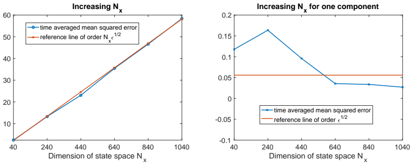
The central claim, stated as Theorem 3.6, is that under short-range interactions, complete observations, and a diagonally dominant localization matrix, the localized Ensemble Kalman-Bucy filter error in each coordinate satisfies $\mathbb{E}[[e_t]_i^2] \leq C\sqrt{\epsilon}$ once $t$ is past a burn-in, that the Laplace transform $\mathbb{E}\exp(\lambda [e_t]_i^2)$ stays bounded for $\lambda$ up to $c\epsilon^{-1/2}$, and that $\mathbb{E}_{t_0}[\sup_{t_0\leq t\leq T}[e_t]_i^2] \leq \max_i\{[e_{t_0}]_i^2\} + C\sqrt{\epsilon}\log(T/\sqrt{\epsilon})$. The $\ell^2$-norm version has total error of order $N_x\sqrt{\epsilon}$, which is what one would expect if the $N_x$ components behave as independent local filters; the novelty is that no individual component's error degrades as $N_x$ grows. The paper further obtains covariance bounds independent of ensemble size $M$, the main obstruction removed by localization, and proves the filter is well-posed for all time as long as the initial covariance has positive diagonal entries.
Load-bearing premise
The results stand or fall on Assumption 3.5: the localization matrix must be diagonally dominant, meaning for each row the off-diagonal weights sum to below 1, and every model interaction must be no stronger than a constant times the localization weight, so that physical interactions cannot extend beyond the localization radius.
Editorial extensions
If this is right
- With $M=10$ ensemble members, the paper's numerical tests on the stochastic Lorenz 96 model show time-averaged per-component error staying flat as $N_x$ increases from 40 to 1040, while the total $\ell^2$ error grows linearly with $N_x$.
- The $\sqrt{\epsilon}$ scaling matches the optimal Kalman-Bucy limit, so reducing observation noise by a factor of four halves the expected component error.
- The $\log(T/\sqrt{\epsilon})$ pathwise bound means a long assimilation window costs only a logarithmic factor in the worst error over the window.
- Covariance entries are bounded above and below by constants of order $\sqrt{\epsilon}$ independent of ensemble size $M$, so the filter neither blows up nor collapses for small observation noise.
- The filter is well defined for all positive times whenever the initial ensemble has positive diagonal covariance entries, even when the ensemble is much smaller than the state dimension.
Reading between the lines
- The diagonal-dominance requirement restricts the compactly supported localization function used in the paper to radius $l\le 1.4$; testing larger radii on systems whose physical interactions stay short-range would show whether the dimension-free bound is a necessary threshold or a proof artifact.
- The Markov-chain construction of the Lyapunov weights suggests a general recipe: any filter whose covariance update respects a Schur-product localization structure may inherit dimension-free error bounds, for instance localized square-root filters or particle filters.
- The paper's setup assumes complete observations on every component via the transformation to $H=I$; a natural stress test is partial or sparse observations, where that transformation fails and one can check whether localization alone still suppresses dimension dependence.
- The logarithmic time dependence and the Gaussian mean-field limit suggest the long-time error resembles a collection of nearly independent local one-dimensional filters; if so, the pathwise bound might be sharpened to replace the $\log(T/\sqrt{\epsilon})$ factor by a dimension-free constant plus a small term.
Signed reviews
Editorial analysis
A structured set of objections, weighed in public.
Referee Report
Summary. The paper analyzes a localized deterministic ensemble Kalman-Bucy filter (l-EnKBF) for continuous-time filtering with full-rank observations and small observation noise. The authors first prove uniform upper and lower bounds on the sample covariance, then derive l2 error bounds of order √ε (up to a factor of the state dimension Nx) together with Laplace-transform bounds, and then, under a diagonal-dominance assumption on the localization matrix and an interaction-domination condition, obtain component-wise error bounds independent of Nx and a pathwise bound whose time growth is only logarithmic. The theoretical exponents are tested on the Lorenz 96 model.
Significance. If the results are valid, the component-wise dimension-independent bounds and the logarithmic pathwise time growth constitute a substantial step beyond earlier linear analyses and beyond the non-localized analysis in [5]. The proof structure is transparent, the bounds are explicit up to constants that are not fitted in the numerics, and the numerical comparisons use theoretical slopes rather than calibrated parameters, which is appropriate. The covariance-matrix lower bound independent of the ensemble size M is also a notable and nontrivial contribution. However, the advertised generality of the main theorems is currently not supported because of an algebraic error in the reduction to unit state noise, and the component-wise result is more restricted than the abstract suggests.
major comments (2)
- [Section 2.2, Eq. (10)] The claimed reduction to σ=I is algebraically incorrect. With \tilde X_t = σ^{-1}X_t, Itô's formula gives d\tilde X_t = σ^{-1}f(X_t)dt + √2 σ^{-1/2}dW_t, not √2 dW_t, because the diffusion coefficient in (1) is √(2σ). The correct whitening transformation is \tilde X_t = σ^{-1/2}X_t; in that case the observation transformation \tilde Y_t = σ^{-1/2}H^-Y_t yields an observation noise covariance σ^{-1/2}H^-RR^TH^{-T}σ^{-1/2} that is not generally diagonal. Since Assumption 2.3 postulates both unit state noise and a diagonal \Omega, the transformation does not reduce the general problem to Assumption 2.3. Consequently Theorems 3.4 and 3.6 are established only for models that already satisfy Assumption 2.3, and the abstract's claim of 'no sacrifice of generality' for arbitrary positive definite σ is unsupported.
- [Section 3.3, Assumption 3.5] The compatibility condition F_{d(i,j)} ≤ C_F φ_{i,j} together with diagonal dominance is substantially more restrictive than the abstract's phrase 'short-range interactions' suggests. Because standard localization functions have compact support, the condition forces all interactions to lie inside the support of φ; for the Gaspari–Cohn function the manuscript itself notes that diagonal dominance requires l ≤ 1.4. Thus Theorem 3.6 only applies when the interaction range is shorter than the localization radius, which is precisely the regime where localization is most benign. This limitation should be stated in the abstract and conclusion, not only in Section 3.3.
minor comments (3)
- [Section C.2, proof of Theorem 3.6, Claim 4] The displayed final inequality in the proof of Claim 4 contains a term 'log Nx' without the factor 1/λ. As written this term does not vanish as ε→0 and would not match the theorem statement; it should be (1/λ)log Nx, which is consistent with the stated C√ε log(NxT/√ε) bound after taking λ = Θ(ε^{-1/2}).
- [Section 4] The numerical experiments simulate the untruncated Lorenz 96 model (14), whereas Assumption 2.1 is verified only for the truncated version (16). The expectation that the two systems behave similarly is plausible, but since the theory requires Assumption 2.1 this should be stated explicitly as an additional assumption rather than asserted by expectation.
- [Section 4.2, Eq. (17)] The notation in Eq. (17), (1/T)∑_{t=1}^T [e_t]^2_i(t), uses t both as a time label in [e_t]^2_i and as a summation index; a different index, such as [e_{t_k}]^2_i, would be clearer.
Circularity Check
No circularity: the dimension-independent error bounds are proved from explicit Lyapunov and Grönwall estimates, with no fitted constants; prior self-citations are contextual.
full rationale
The derivation chain is self-contained at the theorem level. Lemmas 3.1 and 3.2 prove Θ(√ε) upper/lower covariance bounds directly from Assumptions 2.1 and 2.3; Lemma B.1 derives the component-wise error evolution from Itô's formula and Assumption 2.1; Theorem 3.4 and Theorem 3.6 then use Grönwall-type inequalities and the Markov-chain weight construction of Lemma C.1. No parameter is fitted to the quantities being 'predicted': λmax, λmin, β*, and α* are explicit constants, and the numerical section verifies theoretical slopes (e.g., 'reference line of order 1/2') rather than fitting them. The citations to [5]—for the mean-field limit and for the 'same proof' of well-posedness in Corollary 3.3—are prior-work citations that do not smuggle in the dimension-independent or log-T results; Corollary 3.3 is a supporting existence statement and is not used to define the error bounds. Assumption 3.5 is a stated hypothesis (diagonal dominance and F ≤ C_F φ) whose restricted range, e.g. Gaspari–Cohn l ≤ 1.4, is explicitly acknowledged, so it is an applicability restriction, not a circular input. Finally, Section 2.2's 'there is no sacrifice of generality' passage is scale-wise suspect—σ^{-1}X leaves √2 σ^{-1/2}dW rather than √2 dW unless σ = I—but this is a correctness concern about the reduction, not a circularity: it does not make any output equal to an input by construction. No circular step was found.
Assumptions & free parameters
assumptions (5)
- domain assumption Assumption 2.1: the drift f has short-range interactions with Lipschitz constants F_k such that C_f = max_i sum_j F_{d(i,j)} is independent of N_x.
- domain assumption Assumption 2.3: after transformation, the signal noise is identity, the observation operator is identity, and Ω = ε(RR^T)^{-1} is diagonal with ω_min I ≼ Ω ≼ ω_max I.
- domain assumption Assumption 3.5: φ is diagonally dominant and F_{d(i,j)} ≤ C_F φ_{i,j}.
- domain assumption Initial ensemble satisfies ‖P_0‖_min > 0.
- standard math Standard stochastic calculus (Itô, Gronwall, Dynkin) and existence of strong solutions for the SDEs.
Cite this review
Pith. "Pith review of Analysis of a localised nonlinear Ensemble Kalman Bucy Filter with complete and accurate observations." pith.science (2026). https://pith.science/paper/BTWLW7VI
@misc{pith2026190810580,
  author       = {Pith},
  title        = {Pith review of: Analysis of a localised nonlinear Ensemble Kalman Bucy Filter with complete and accurate observations},
  year         = {2026},
  howpublished = {\url{https://pith.science/paper/BTWLW7VI}},
  note         = {Machine review of arXiv:1908.10580}
}
read the original abstract
Concurrent observation technologies have made high-precision real-time data available in large quantities. Data assimilation (DA) is concerned with how to combine this data with physical models to produce accurate predictions. For spatial-temporal models, the Ensemble Kalman Filter with proper localization techniques is considered to be a state-of-the-art DA methodology. This article proposes and investigates a localized Ensemble Kalman Bucy Filter (l-EnKBF) for nonlinear models with short-range interactions. We derive dimension-independent and component-wise error bounds and show the long time path-wise error only has logarithmic dependence on the time range. The theoretical results are verified through some simple numerical tests.
Figures


Reference graph
Works this paper leans on
-
[5]
Jana de Wiljes, Sebastian Reich, and Wilhelm Stannat. Long-time st ability and accuracy of the ensemble Kalman-Bucy filter for fully observed processes and small measure ment noise. Siam J. Applied Dynamical Systems, 17(2):1152–1181, 2018
work page 2018
-
[1]
J. Amezcua, E. Kalnay, K. Ide, and S. Reich. Ensemble transfor m Kalman-Bucy filters. Q.J.R. Meteor. Soc., 140:995–1004, 2014
work page 2014
-
[2]
K. Bergemann and S. Reich. An ensemble Kalman-Bucy filter for co ntinuous data assimilation. Meteorolog. Zeitschrift, 21:213–219, 2012. 22
work page 2012
-
[3]
P. J. Bickel and E. Levina. Regularized estimation of large covaria nce matrices. The Annals of Statistics, 36(1):199–227, 2008
work page 2008
-
[4]
A. N. Bishop and P. Del Moral. On the stability of Kalman-Bucy diffus ion. SIAM J. Control and Optimization, 55(6):4015–4047, 2017
work page 2017
-
[6]
P. Del Moral and J. Tugaut. On the stability and the uniform prop agation of chaos properties of ensemble Kalman-Bucy filters. Ann. Appl. Probab., 28(2):790–850, 2018
work page 2018
-
[7]
G. Evensen. Data Assimilation: The Ensemble Kalman Filter. Springer, 2006
work page 2006
-
[8]
Large sample asymptotics for the ensemble kalman filter
Vu-Duc Tran Fran¸ cois Le Gland, Valerie Monbet. Large sample asymptotics for the ensemble kalman filter. inria-00409060 pp.25., RR-7014, INRIA, 2009
work page 2009
Show all 32 references
-
[9]
Gaspari and S.E
G. Gaspari and S.E. Cohn. Construction of correlation function s in two and three dimensions. Q. J. Royal Meteorological Soc., 125:723–757, 1999
1999
-
[10]
H ˙ akon Hoel, Kody J. H. Law, and Raul Tempone. Multilevel ense mble Kalman filtering. SIAM Journal on Numerical Analysis, 54(3):1813–1839, 2016
2016
-
[11]
Mult ilevel ensemble Kalman filtering with local-level Kalman gains
H ˙ akon Hoel, Gaukhar Shaimerdenova, and Raul Tempone. Mult ilevel ensemble Kalman filtering with local-level Kalman gains. https://arxiv.org/abs/2002.00480, 2020
2002 arXiv
-
[12]
Jazwinski
A.H. Jazwinski. Stochastic processes and filtering theory. Academic Press, New York, 1970
1970
-
[13]
R. E. Kalman. A new approach to linear filtering and prediction pro blems. Transaction of the ASME Journal of Basic Engineering, pages 35–45, 1960
1960
-
[14]
E. Kalnay. Atmospheric modeling, data assimilation and predictability. Cambridge University Press, 2002
2002
-
[15]
Kelly, A.J
D. Kelly, A.J. Majda, and X.T. Tong. Concrete ensemble Kalman filt ers with rigorous catastrophic filter divergence. Proc. Natl. Acad. Sci. USA, 112:10589–10594, 2015
2015
-
[16]
D. T. Kelly, K. J. H. Law, and A. Stuart. Well-posedness and acc uracy of the ensemble Kalman filter in discrete and continuous time. Nonlinearity, 27:2579–2604, 2014
2014
-
[17]
Convergence of the square root ensemble kalman filter in the large ensemble limit
Evan Kwiatkowski and Jan Mandel. Convergence of the square root ensemble kalman filter in the large ensemble limit. SIAM/ASA Journal on Uncertainty Quantification, 3(1):1–17, 2015
2015
-
[18]
On the continuous time limit of ensemble square root filters
Theresa Lange and Wilhelm Stannat. On the continuous time limit of ensemble square root filters. arXiv:1910.12493, 2019
1910 arXiv
-
[19]
Kody J. H. Law, Hamidou Tembine, and Raul Tempone. Determinis tic mean-field ensemble kalman filter- ing. SIAM Journal on Scientific Computing, 38(3):A1251–A1279, 2016
2016
-
[20]
E.N. Lorenz. Predictibility: A problem partly solved. In Proc. Seminar on Predictibility, volume 1, pages 1–18, ECMWF, Reading, Berkshire, UK, 1996
1996
-
[21]
Majda and X
A. Majda and X. T. Tong. Performance of ensemble Kalman filter s in large dimensions. Communications on Pure and Applied Mathematics, 71(5):892–937, 2018
2018
-
[22]
Mandel, L
J. Mandel, L. Cobb, and J. D. Beezley. On the convergence of t he ensemble Kalman filter. Applications of Mathematics, 56(6):533–541, 2011
2011
-
[23]
Jan Mandel, Loren Cobb, and Jonathan D. Beezley. On the conv ergence of the ensemble kalman filter. Applications of Mathematics, 533-541:533–541, 2011
2011
-
[24]
Morzfeld, X.T
M. Morzfeld, X.T. Tong, and Y.M. Marzouk. Localization for MCMC : sampling high-dimensional posterior distributions with local structure. J. Comput. Phys., 310:1–28, 2019. 23
2019
-
[25]
Oliver, A
D. Oliver, A. Reynolds, and N. Liu. Inverse Theory for Petroleum Reservoir Characterization and History Matching. Cambridge University Press, 2008
2008
-
[26]
S. Reich. A nonparametric ensemble transform method for Bay esian inference. SIAM J. Sci. Comput., 35:A2013–A2024, 2013
2013
-
[27]
Reich and C.J
S. Reich and C.J. Cotter. Probabilistic Forecasting and Bayesian Data Assimilation. Cambridge University Press, Cambridge, 2015
2015
-
[28]
Cambridge University Press, 2013
Simo S¨ arkk¨ a.Bayesian Filtering and Smoothing. Cambridge University Press, 2013
2013
-
[29]
X.T. Tong. Performance analysis of local ensemble Kalman filter. J. Non. Sci., 28(4):1397–1442, 2018
2018
-
[30]
Tong, A.J
X.T. Tong, A.J. Majda, and D. Kelly. Nonlinear stability and ergodic ity of ensemble based Kalman filters. Nonlinearity, 29(2):657, 2016
2016
-
[31]
X.T. Tong, M. Morzfeld, and Y.M. Marzouk. MALA-within-Gibbs sa mplers for high-dimensional distri- butions with sparse conditional structure. accepted by SIAM Jou rnal on Scientific Computing, arXiv: 1908.09429, 2020
1908 arXiv
-
[32]
Yang, P.G
T. Yang, P.G. Mehta, and S.P. Meyn. Feedback particle filter. IEEE Trans. Automatic Control, 58:2465– 2480, 2013. 24
2013
Reviewed August 14, 2026 · model on record in the stance chip above.
Discussion (0). Continue with ORCID to comment.