REVIEW 2 major objections 3 minor 1 cited by
Monotone Contractions
T0 review · 2 major / 3 minor · reviewed 2026-08-12 · deepseek-v4-flash
Pith's one-line read A monotone contraction in three dimensions admits an O(log(1/ε))-query algorithm for ε-approximate fixed points, and the problem lies in UEOPL.
desk verdict Strong, novel results for monotone contractions, but the 3D algorithm's keystone Lemma 84 misuses Lemma 80, so the O(log(1/ε)) query bound is not yet proven. read the letter →
The pith
A machine-rendered reading of the paper's core claim, the machinery that carries it, and where it could break.
The reading
What carries the argument
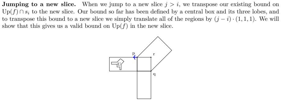
The load-bearing objects are the discrete monotone approximate contraction (DMAC) instance, its one-dimensional surfaces, and the critical boxes used to bound the up-set in a two-dimensional slice. A surface is the unique height at which a fixed one-dimensional slice is stationary; in a violation-free instance every surface is monotone and has gradient at most one, which lets bounds be translated diagonally from one slice to the next. A critical box is a rectangle inside the up-set whose right, top, and lower-left exits all move strictly downward, so the box together with its left, bottom, and diagonal lobes contains the whole up-set; the almost-square lemma says a critical box with $\lvert h-w\rvert\le 1$ exists whenever the up-set is non-empty. The UEOPL containment is carried by a promise-preserving reduction to One Permutation Discrete Contraction (OPDC), using the least-fixed-point verification sequence and mapping every OPDC violation back to a monotonicity or non-expansion violation of DMAC.
What would settle it
Enumerate all monotone non-expansive displacement fields on a small grid, say $5\times 5\times 5$, with inward boundary behavior and test Lemma 81: a single slice whose up-set is non-empty but whose every critical box satisfies $\lvert h-w\rvert\ge 2$ would falsify the 3D query bound. Alternatively, implement the algorithm on a family of monotone contractions built by rotating the displacement field by 90 degrees and check whether the carried-over bounds shrink by a constant fraction at each slice; a failure would show the carried-over bound lemma is false.
Extended reading notes
Core claim
On the paper's own terms, the discovery is that combining monotonicity with contraction makes fixed-point search structurally easier than either condition alone. The paper defines DMAC, a discrete function on a grid with unit displacements that can output a fixed point, a monotonicity violation, or a non-expansion violation, reduces monotone contractions to it, and proves DMAC lies in UEOPL by selecting the least fixed point as the unique solution. The least fixed point is efficiently verifiable because a non-least fixed point is always approached by another fixed point one unit away, so a short verification sequence certifies it. The algorithmic core is a 3D DMAC solver that maintains a bound on the up-set made of a critical box and three lobes, shrinks the bound by a constant fraction per query using grid searches, cone arguments, and bounds carried between slices, and finishes with a terminal phase on a slice that contains a fixed point. The decomposition theorem then multiplies this 3D solver to higher dimensions.
Load-bearing premise
The constant-factor shrinking step works only if every nonempty up-set in a two-dimensional slice contains a critical box whose height and width differ by at most one (Lemma 81); if that fails, the per-query progress guarantee and the $O(\log(1/\varepsilon))$ query count collapse.
Editorial extensions
If this is right
- A 3D monotone contraction admits an $\varepsilon$-approximate fixed point with $O(\log(1/\varepsilon))$ function evaluations, each evaluation processed in polynomial time.
- For $d$ dimensions the same construction needs $O((c\log(1/\varepsilon))^{\lceil d/3\rceil})$ evaluations and runs in polynomial time per step, improving the previous $O((c\log(1/\varepsilon))^{\lceil d/2\rceil+1})$ polynomial-time bound for monotone functions.
- Approximating the value of a Shapley stochastic game with $d$ states lies in UEOPL and can be done in time $O((c\log(1/\varepsilon))^{\lceil d/3\rceil}\cdot \mathrm{poly}(|G|))$.
- For functions that are only contracting and not monotone, the best polynomial-time algorithms need $\log^d(1/\varepsilon)$ evaluations, so monotonicity removes nearly all of the dimension dependence in the exponent.
- The least fixed point of a DMAC instance can be verified in polynomial time, in contrast to monotone functions alone, where the same verification is NP-hard even in one-dimensional instances.
Reading between the lines
- The paper does not claim a matching lower bound; if the 3D base case is optimal, the decomposition theorem makes $\lceil d/3\rceil$ the bottleneck, so any faster general algorithm would need a better 3D fixed-point search rather than a better composition.
- A continuous analogue of the almost-square critical box lemma would remove the discretization slack in the reduction from monotone contractions to DMAC; whether the exact-square version holds in $\mathbb{R}^3$ is not addressed by the paper.
- The promise-preserving reduction means the algorithm could serve as a violation detector for purported monotone contractions: if the produced OPDC instance reports a violation, the original function provably violates monotonicity or non-expansion, even though the paper states this only in complexity-theoretic terms.
Signed reviews
Editorial analysis
A structured set of objections, weighed in public.
Referee Report
Summary. This paper studies functions f : [0,1]^d → [0,1]^d that are both monotone and contracting in the ℓ∞ norm. It defines the discrete problem DMAC and claims three main results: (1) DMAC and hence MonotoneContraction lie in UEOPL via a promise-preserving reduction to OPDC; (2) a three-dimensional DMAC instance can be solved with O(log n) queries, where n = Ω(1/ε), with each step polynomial time; and (3) a decomposition theorem converts any LFP-solver in dimensions d1 and d2 into one in dimension d1+d2, yielding an O((c log(1/ε))^{⌈d/3⌉})-query algorithm in dimension d. The results are applied to Shapley stochastic games. The most intricate part is Section 8, which gives the three-dimensional algorithm; Section 8.3 develops the almost-square critical box lemma (Lemma 81) on which the query-count argument rests. In the version under review, the proof of Lemma 81 is cut off and the preceding Lemma 84 relies on a misstatement of Lemma 80. The earlier sections (4–7) are detailed and, as far as I checked, internally coherent.
Significance. If the Section 8.3 concerns are resolved, the results would be a substantial improvement over the previous state of the art: they place monotone-contraction fixed-point finding in UEOPL (not previously known), reduce the query complexity from O(log^{⌈d/2⌉}(1/ε)) to O((c log(1/ε))^{⌈d/3⌉}), and the per-step polynomial runtime addresses the drawback of Chen et al.'s O(d² log(1/ε))-query algorithm. The paper is genuinely strong in several places: the contiguity proof for fixed points (Lemma 17), the polynomial-time least-fixed-point verification (Lemma 19), the reduction to OPDC with violation handling (Section 5.3), the 1DUniqueDMAC reduction and surface characterization (Section 6), and the decomposition theorem (Section 7.1) are all carefully presented with detailed arguments. The main doubt sits at the keystone of the algorithm: Section 8.3's claim that an almost-square critical box always exists. Because the query complexity of the grid-search subroutines depends on that lemma, the algorithmic main claims are conditional on a repair of the issues I identify.
major comments (2)
- [8.3, Lemma 84] The proof of Lemma 84 states that 'Lemma 80 tells us that if f3(x) > x3 and if y ≤ x then f3(y) > y3' and uses this to conclude that the set D of points with f3(x) > x3 is downward closed. This inverts the hypotheses of Lemma 80: the third bullet of Lemma 80 requires y ≥ x and yi = xi, not y ≤ x. Consequently, the conclusion 'x ≥ y for all points y ∈ B' is not established, and the construction of a point in Up(f) ∩ B fails. Since Lemma 84 is the starting point of the intermediate-value argument in Lemma 87, and Lemma 87 is used in the proof of Lemma 81, the existence of an almost-square critical box—used in Sections 8.4–8.6 to justify the constant-size grid search—is not proven. This is load-bearing for the O(log n) query claim.
- [8.3, Lemma 81 proof] In the version provided, the proof of Lemma 81 ends mid-sentence with '≤ Height1(xi+1) + 1 − (Hei', cutting off in the middle of the case analysis for xi+1 = xi + e1 and before the case xi+1 = xi − e2 is presented. The reader cannot check the claimed reductions of Height1/Height2 or the resulting construction of the almost-square box. Combined with the flaw in Lemma 84, the statement 'If Up(f) ∩ s is non-empty then there exists a critical box with |h−w| ≤ 1' is unsupported in this version. Please provide the full proof or repair the argument.
minor comments (3)
- [6.3, proof of Lemma 71] The text says 'the reduction is correct for the case when x3 = 1 and x1 > n', but the lemma requires x1 > 1; the variable x1 ranges only up to n in G′. This appears to be a typo that could mislead readers.
- [7.2, Step 1] Figures 16 and 17 are referenced in the interpolation description, but the figures are not included in the text I reviewed; the claim that the surfaces match on cube boundaries and that the gradients are at most one cannot be fully checked in their absence.
- [Footnote 5] The word 'analagously' should be 'analogously'.
Circularity Check
No significant circularity: results are derived against external OPDC/UEOPL benchmarks; self-citations supply independent prior theorems.
full rationale
The paper's central claims (UEOPL containment, the O(log(1/ε)) 3D query bound, and the decomposition theorem) are derived from the definitions of monotone contractions and the discrete DMAC problem, not from the conclusions they are meant to establish. The reduction from MonotoneContraction to DMAC defines f from g by clamping displacements, and each solution type of the DMAC instance is mapped back to the corresponding solution of MonotoneContraction by explicit inequalities (Lemmas 6-9); this is a standard reduction, not a definitional equivalence between the target and the algorithm's output. The UEOPL containment is obtained by a reduction to OPDC, whose UEOPL-completeness is cited from prior work [14] by overlapping authors; that prior theorem is an independent, parameter-free result about a different problem and is not fed by the present paper's fitted values or assumptions, so it is real evidence rather than circularity. Similarly, Lemma 67 is cited from [15] as a standard monotone-function interpolation lemma, and the decomposition theorem is proved directly for LFP-solving algorithms. No parameter is fitted and then renamed as a prediction, and no 'uniqueness' choice is forced by a self-citation chain. The only concerns raised about Lemma 84 are potential mathematical gaps in the proof of an almost-square critical box; even if valid, such a flaw would be a correctness issue, not a circularity. The derivation chain is therefore self-contained against external benchmarks.
Assumptions & free parameters
assumptions (6)
- standard math Tarski's (Knaster-Tarski) fixed point theorem: every order-preserving map on a complete lattice has a least fixed point.
- standard math Banach fixed point theorem: a contraction on a complete metric space has a unique fixed point.
- domain assumption OPDC is UEOPL-complete (Fearnley, Gordon, Mehta, Savani 2019).
- domain assumption Shapley stochastic games reduce to monotone contractions (Etessami et al. 2008).
- domain assumption Monotone functions satisfy a sandwich fixed-point lemma (Fearnley et al., Lemma 3.2 of [15]).
- domain assumption DMAC instances can be assumed to have unit-length displacements (Lemma 11) and are represented by a polynomial-time Turing machine.
Cite this review
Pith. "Pith review of Monotone Contractions." pith.science (2026). https://pith.science/paper/BUZRCHFY
@misc{pith2026241110107,
  author       = {Pith},
  title        = {Pith review of: Monotone Contractions},
  year         = {2026},
  howpublished = {\url{https://pith.science/paper/BUZRCHFY}},
  note         = {Machine review of arXiv:2411.10107}
}
abstract
We study functions $f : [0, 1]^d \rightarrow [0, 1]^d$ that are both monotone and contracting, and we consider the problem of finding an $\varepsilon$-approximate fixed point of $f$. We show that the problem lies in the complexity class UEOPL. We give an algorithm that finds an $\varepsilon$-approximate fixed point of a three-dimensional monotone contraction using $O(\log (1/\varepsilon))$ queries to $f$. We also give a decomposition theorem that allows us to use this result to obtain an algorithm that finds an $\varepsilon$-approximate fixed point of a $d$-dimensional monotone contraction using $O((c \cdot \log (1/\varepsilon))^{\lceil d / 3 \rceil})$ queries to $f$ for some constant $c$. Moreover, each step of both of our algorithms takes time that is polynomial in the representation of $f$. These results are strictly better than the best-known results for functions that are only monotone, or only contracting. All of our results also apply to Shapley stochastic games, which are known to be reducible to the monotone contraction problem. Thus we put Shapley games in UEOPL, and we give a faster algorithm for approximating the value of a Shapley game.
Figures


Figures from the paper (39 more)








Forward citations
Cited by 1 Pith paper
-
ARRIVAL: Recursive Framework & $\ell_1$-Contraction
An algorithm solves ARRIVAL in time 2^{O(k log^2 n)} on n-vertex graphs of treewidth k, and G-ARRIVAL reduces to finding approximate fixed points of l1-contractions.
Reference graph
Works this paper leans on
-
[1]
Sur les opérations dans les ensembles abs traits et leur application aux équations intégrales
Stefan Banach. Sur les opérations dans les ensembles abs traits et leur application aux équations intégrales. Fundamenta mathematicae, 3(1):133–181, 1922. 85
work page 1922
-
[2]
Boonyasiriwat, Kris Sikorski, and Ch
Ch. Boonyasiriwat, Kris Sikorski, and Ch. Xiong. A note o n two fixed point problems. J. Complexity, 23(4-6):952–961, 2007
work page 2007
-
[3]
Improved upper bounds for finding Tar ski fixed points
Xi Chen and Yuhao Li. Improved upper bounds for finding Tar ski fixed points. In Proc. of EC , pages 1108–1118, 2022
work page 2022
-
[4]
Reducing Tars ki to unique Tarski (in the black-box model)
Xi Chen, Yuhao Li, and Mihalis Yannakakis. Reducing Tars ki to unique Tarski (in the black-box model). In Proc. of CCC , volume 264 of LIPIcs, pages 21:1–21:23, 2023
work page 2023
-
[5]
Computing a fix ed point of contraction maps in polynomial queries
Xi Chen, Yuhao Li, and Mihalis Yannakakis. Computing a fix ed point of contraction maps in polynomial queries. In Proc. of STOC , pages 1364–1373, 2024
work page 2024
-
[6]
Computations and com plexities of Tarski’s fixed points and supermodular games
Chuangyin Dang, Qi Qi, and Yinyu Ye. Computations and com plexities of Tarski’s fixed points and supermodular games. CoRR, abs/2005.09836, 2020. Stanford tech report version appea red in 2012
arXiv 2005
-
[7]
Constantinos Daskalakis and Christos H. Papadimitriou . Continuous local search. In Proc. of SODA, pages 790–804, 2011
work page 2011
-
[8]
A Converse to Banach’s Fixed Point Theorem and its CLS Completeness
Constantinos Daskalakis, Christos Tzamos, and Manolis Zampetakis. A Converse to Banach’s Fixed Point Theorem and its CLS Completeness. In Proc. of STOC , pages 44–50, 2018
work page 2018
Show all 28 references
-
[9]
Papadimitriou, A viad Rubi nstein, and Mihalis Yannakakis
Kousha Etessami, Christos H. Papadimitriou, A viad Rubi nstein, and Mihalis Yannakakis. Tarski’s theorem, supermodular games, and the complexity of equilib ria. In Proc. of ITCS , volume 151 of LIPIcs, pages 18:1–18:19, 2020
2020
-
[10]
On the complex ity of nash equilibria and other fixed points
Kousha Etessami and Mihalis Yannakakis. On the complex ity of nash equilibria and other fixed points. SIAM J. Comput. , 39(6):2531–2597, 2010
2010
-
[11]
The complexity of gradient descent: CLS = PPAD ∩ PLS
John Fearnley, Paul Goldberg, Alexandros Hollender, a nd Rahul Savani. The complexity of gradient descent: CLS = PPAD ∩ PLS. J. ACM, 70(1):7:1–7:74, 2023
2023
-
[12]
CLS: New problems and complete- ness
John Fearnley, Spencer Gordon, Ruta Mehta, and Rahul Sa vani. CLS: New problems and complete- ness. CoRR, abs/1702.06017, 2017
2017 arXiv
-
[13]
Unique end of potential line
John Fearnley, Spencer Gordon, Ruta Mehta, and Rahul Sa vani. Unique end of potential line. In Proc. of ICALP , volume 132, pages 56:1–56:15, 2019. https://arxiv.org/abs/1811.03841
2019 arXiv
-
[14]
Unique end of potential line
John Fearnley, Spencer Gordon, Ruta Mehta, and Rahul Sa vani. Unique end of potential line. J. Comput. Syst. Sci. , 114:1–35, 2020
2020
-
[15]
A f aster algorithm for finding Tarski fixed points
John Fearnley, Dömötör Pálvölgyi, and Rahul Savani. A f aster algorithm for finding Tarski fixed points. ACM Trans. Algorithms, 18(3):23:1–23:23, 2022
2022
-
[16]
Tsi- garidas
Kristoffer Arnsfelt Hansen, Michal Koucký, Niels Lauri tzen, Peter Bro Miltersen, and Elias P. Tsi- garidas. Exact algorithms for solving stochastic games: ex tended abstract. In Proc. of STOC , pages 205–214, 2011
2011
-
[17]
Tsi- garidas
Kristoffer Arnsfelt Hansen, Michal Koucký, Niels Lauri tzen, Peter Bro Miltersen, and Elias P. Tsi- garidas. Exact algorithms for solving stochastic games. CoRR, abs/1202.3898, 2012
2012 arXiv
-
[18]
Huang, Leonid G
Z. Huang, Leonid G. Khachiyan, and Christopher (Krzysz tof) Sikorski. Approximating fixed points of weakly contracting mappings. J. Complexity , 15(2):200–213, 1999
1999
-
[19]
Prism-games 3.0: Stochas- tic game verification with concurrency, equilibria and time
Marta Kwiatkowska, Gethin Norman, David Parker, and Ga briel Santos. Prism-games 3.0: Stochas- tic game verification with concurrency, equilibria and time . In Proc. of CAV , volume 12225, pages 475–487, 2020
2020
-
[20]
New algorithms for solving zero-s um stochastic games
Miquel Oliu-Barton. New algorithms for solving zero-s um stochastic games. Math. Oper. Res. , 46(1):255–267, 2021
2021
-
[21]
Llloyd S. Shapley. Stochastic games*. Proceedings of the National Academy of Sciences , 39(10):1095– 1100, 1953
1953
-
[22]
Shellman and Christopher (Krzysztof) Sikor ski
Spencer D. Shellman and Christopher (Krzysztof) Sikor ski. A recursive algorithm for the infinity- norm fixed point problem. J. Complex. , 19(6):799–834, 2003. 86
2003
-
[23]
Shellman and Kris Sikorski
Spencer D. Shellman and Kris Sikorski. A two-dimension al bisection envelope algorithm for fixed points. J. Complexity , 18(2):641–659, 2002
2002
-
[24]
Shellman and Kris Sikorski
Spencer D. Shellman and Kris Sikorski. Algorithm 825: A deep-cut bisection envelope algorithm for fixed points. ACM Trans. Math. Softw. , 29(3):309–325, 2003
2003
-
[25]
Shellman and Kris Sikorski
Spencer D. Shellman and Kris Sikorski. Algorithm 848: A recursive fixed-point algorithm for the infinity-norm case. ACM Trans. Math. Softw. , 31(4):580–586, 2005
2005
-
[26]
Computational complexity of fixed points
Krzysztof Sikorski. Computational complexity of fixed points. Journal of Fixed Point Theory and Applications, 6(2):249–283, 2009
2009
-
[27]
Stochastic games
Eilon Solan and Nicolas Vieille. Stochastic games. Proceedings of the National Academy of Sciences , 112(45):13743–13746, 2015
2015
-
[28]
A lattice-theoretical fixpoint theorem and its applications
Alfred Tarski. A lattice-theoretical fixpoint theorem and its applications. Pacific Journal of Mathe- matics, 5(2):285–309, 1955. 87
1955
Reviewed August 12, 2026 · model on record in the stance chip above.
Discussion (0). Continue with ORCID to comment.