Low Stage High Order Explicit Runge--Kutta Methods via Q- and D-Conditions: General Theory and Efficient Recursive Construction
Pith reviewed 2026-05-19 19:10 UTC · model grok-4.3
The pith
A Q/D-space reformulation of order conditions yields explicit Runge-Kutta methods of even order p with stage count (p squared minus 2p plus 8) over 4.
A machine-rendered reading of the paper's core claim, the machinery that carries it, and where it could break.
Core claim
The Q- and D-space residual conditions together with B(p) form a set of sufficient conditions that guarantee order p for an explicit Runge-Kutta method; the same conditions admit a recursive construction in which the Butcher coefficients are obtained from two structured linear systems, producing, for every even p greater than or equal to 4, a method whose stage count is exactly (p squared minus 2p plus 8) divided by 4.
What carries the argument
The Q- and D-spaces, defined through their residual vectors, which reformulate Butcher's classical simplifying assumptions into a pair of simplified linear spaces whose residuals supply the sufficient order conditions.
If this is right
- For each even p greater than or equal to 4 an explicit Runge-Kutta method of order p exists with stage count (p squared minus 2p plus 8) divided by 4.
- The construction is recursive, so higher-order methods can be built systematically from lower-order ones by solving two linear systems per step.
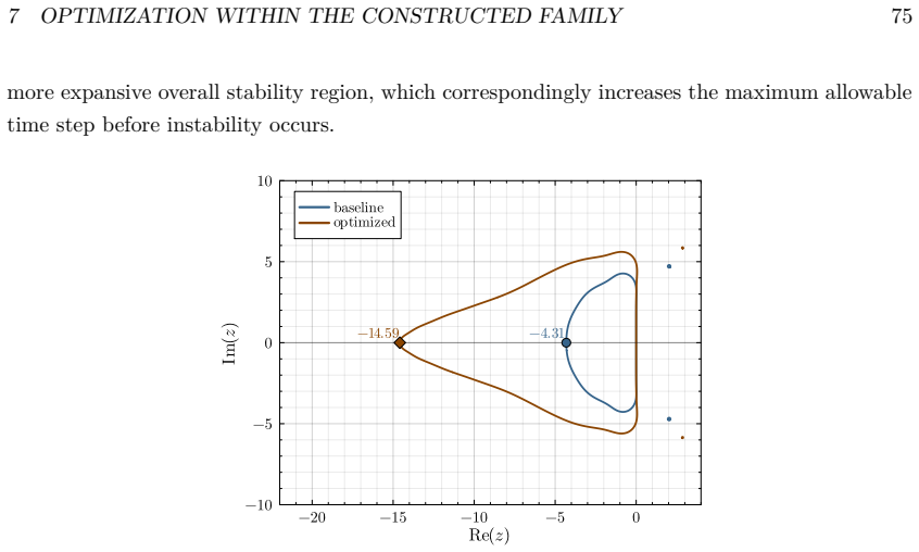
- Free parameters left by the construction can be chosen to improve linear stability or short-time accuracy without losing the guaranteed order.
- The Q/D framework supplies a concrete generalization of Butcher's simplifying assumptions that still guarantees the full order when combined with B(p).
Where Pith is reading between the lines
- The improved linear term in the stage count may translate into lower computational cost per step for problems where function evaluations dominate the runtime.
- The retained free parameters could be optimized for particular classes of problems such as Hamiltonian systems or stiff oscillatory equations.
- Because the construction is recursive, it may be possible to derive families with additional algebraic properties such as symplecticity or preservation of quadratic invariants by imposing extra linear constraints on the free parameters.
Load-bearing premise
The Q- and D-space residual conditions remain linearly independent and the two structured linear systems at each recursive step remain solvable for the chosen stage count.
What would settle it
Explicitly construct the method for p equals 6 using the recursive procedure, insert the resulting Butcher tableau into a test equation with known exact solution, and verify that the observed order of the local truncation error is exactly 6.
Figures




read the original abstract
Constructing explicit Runge--Kutta (ERK) methods with as few stages as possible for a given order is a classical problem in numerical analysis. In this work, we introduce a $Q$/$D$-space framework of sufficient order conditions for ERK methods. This framework generalizes Butcher's classical simplifying assumptions by reformulating them in terms of simplified $Q$- and $D$-spaces defined through their residual vectors. It yields sufficient conditions which, together with $B(p)$, ensure order $p$. It also leads to a recursive construction procedure for ERK methods of arbitrary even order, in which the Butcher coefficients are obtained from two structured linear systems. For every even order $p\ge 4$, the construction produces ERK methods with stage number $s(p)=(p^2-2p+8)/4$. This stage count has the same leading term as that of the classical Gragg families, while improving the linear term. The free parameters retained by the construction further provide a systematic framework for designing methods with enhanced stability and short-time accuracy.
Editorial analysis
A structured set of objections, weighed in public.
Referee Report
Summary. The paper introduces a Q/D-space framework that reformulates Butcher's simplifying assumptions via residual vectors to obtain sufficient order conditions for explicit Runge-Kutta methods. Combined with the classical B(p) condition, these yield order p. The framework supports a recursive construction in which Butcher coefficients are obtained from two structured linear systems at each step. For every even order p ≥ 4 the construction produces methods with stage count s(p) = (p² - 2p + 8)/4, which matches the leading term of the classical Gragg families while improving the linear term; free parameters remain for stability or accuracy tuning.
Significance. If the linear-independence claims hold, the work supplies an algebraic route to explicit Runge-Kutta methods whose stage count is asymptotically optimal among known families and whose construction is fully recursive and parameter-free at the order level. The retention of free parameters after the order conditions are satisfied is a concrete strength that enables systematic optimization of stability regions or short-time accuracy without restarting the order derivation.
major comments (1)
- [§4] §4, recursive step: the solvability of the two structured linear systems at each recursion level is asserted on the basis of linear independence of the Q- and D-residual vectors for the chosen stage count s(p). The manuscript verifies this for base cases and small even p, but does not supply a general rank argument that the coefficient matrices have full row rank equal to the number of imposed conditions for arbitrary even p. Because the stage-count formula s(p) = (p² - 2p + 8)/4 is derived from this count, a missing general independence proof is load-bearing for the central claim.
minor comments (2)
- [§2-4] Notation: the definition of the Q- and D-spaces via residual vectors is introduced in §2 but the precise mapping from residual vectors to the rows of the two linear systems is not restated in §3-4; a short summary table or diagram would improve readability.
- [Abstract] The abstract states that the construction 'yields sufficient conditions which, together with B(p), ensure order p'; this should be cross-referenced to the precise theorem number in the main text.
Simulated Author's Rebuttal
We thank the referee for the positive evaluation of the significance of the Q/D-space framework and for the constructive identification of the need for a general rank argument. We address the single major comment below and will revise the manuscript to incorporate the requested strengthening.
read point-by-point responses
-
Referee: [§4] §4, recursive step: the solvability of the two structured linear systems at each recursion level is asserted on the basis of linear independence of the Q- and D-residual vectors for the chosen stage count s(p). The manuscript verifies this for base cases and small even p, but does not supply a general rank argument that the coefficient matrices have full row rank equal to the number of imposed conditions for arbitrary even p. Because the stage-count formula s(p) = (p² - 2p + 8)/4 is derived from this count, a missing general independence proof is load-bearing for the central claim.
Authors: We agree that the absence of a general proof of full row rank for arbitrary even p constitutes a genuine gap in the current exposition. The manuscript establishes the required linear independence only by direct verification for the base cases p=4 and p=6 together with explicit rank computations for selected larger even orders. In the revised version we will add an inductive argument in §4 showing that the coefficient matrices retain full row rank at every recursion level. The induction proceeds from the block-triangular structure of the Q- and D-residual vectors: each newly introduced stage augments the residual space by a vector whose leading nonzero entry lies outside the span of the preceding residuals, and the specific choice s(p)=(p²-2p+8)/4 guarantees that the number of free parameters is sufficient to maintain this separation. The revised text will include the explicit inductive step together with a short appendix verifying the base of the induction. revision: yes
Circularity Check
No significant circularity; derivation rests on classical B(p) and external linear algebra
full rationale
The paper defines Q- and D-spaces via residual vectors, reformulates Butcher's simplifying assumptions, and states that the resulting conditions plus the classical B(p) are sufficient to guarantee order p. The recursive construction obtains Butcher coefficients by solving two structured linear systems whose dimensions are set by the chosen stage count s(p). No step reduces the order claim or the stage count to a fitted parameter or self-citation by construction; solvability is asserted on the basis of the framework and linear independence of the residual vectors rather than by redefining the target result inside the same equations. The free parameters are explicitly retained for later use and do not enter the order or stage-count claims. The derivation is therefore self-contained against the external benchmarks of Butcher theory and standard linear algebra.
Axiom & Free-Parameter Ledger
axioms (2)
- domain assumption The Q-space and D-space residual vectors remain linearly independent when the stage count is set to (p²-2p+8)/4
- domain assumption B(p) together with the Q/D conditions are sufficient for order p
Lean theorems connected to this paper
-
IndisputableMonolith/Foundation/RealityFromDistinction.leanreality_from_one_distinction unclear?
unclearRelation between the paper passage and the cited Recognition theorem.
Q/D-space framework of sufficient order conditions... recursive construction procedure... s(p)=(p²-2p+8)/4
-
IndisputableMonolith/Cost/FunctionalEquation.leanwashburn_uniqueness_aczel unclear?
unclearRelation between the paper passage and the cited Recognition theorem.
Butcher coefficients obtained from two structured linear systems
What do these tags mean?
- matches
- The paper's claim is directly supported by a theorem in the formal canon.
- supports
- The theorem supports part of the paper's argument, but the paper may add assumptions or extra steps.
- extends
- The paper goes beyond the formal theorem; the theorem is a base layer rather than the whole result.
- uses
- The paper appears to rely on the theorem as machinery.
- contradicts
- The paper's claim conflicts with a theorem or certificate in the canon.
- unclear
- Pith found a possible connection, but the passage is too broad, indirect, or ambiguous to say the theorem truly supports the claim.
Reference graph
Works this paper leans on
-
[1]
Markus Bachmayr, Reinhold Schneider, and André Uschmajew. “Tensor networks and hi- erarchical tensors for the solution of high-dimensional partial differential equations”. In: Foundations of Computational Mathematics 16.6 (2016), pp. 1423–1472
work page 2016
-
[2]
Counting Rooted Trees: The Universal Law t(n) ∼ Cρ −nn−3/2
Jason P Bell, Stanley N Burris, and Karen A Yeats. “Counting Rooted Trees: The Universal Law t(n) ∼ Cρ −nn−3/2”. In: the electronic journal of combinatorics (2006), R63– R63
work page 2006
-
[3]
A 3(2) pair of Runge-Kutta formulas
Przemyslaw Bogacki and Lawrence F Shampine. “A 3(2) pair of Runge-Kutta formulas”. In: Applied Mathematics Letters 2.4 (1989), pp. 321–325
work page 1989
-
[4]
Coefficients for the study of Runge-Kutta integration processes
John C Butcher. “Coefficients for the study of Runge-Kutta integration processes”. In: Journal of the Australian Mathematical Society 3.2 (1963), pp. 185–201
work page 1963
-
[5]
Implicit runge-kutta processes
John C Butcher. “Implicit runge-kutta processes”. In: Mathematics of computation 18.85 (1964), pp. 50–64
work page 1964
-
[6]
On Runge-Kutta processes of high order
John C Butcher. “On Runge-Kutta processes of high order”. In: Journal of the Aus- tralian Mathematical Society 4.2 (1964), pp. 179–194
work page 1964
-
[7]
A history of Runge-Kutta methods
John Charles Butcher. “A history of Runge-Kutta methods”. In: Applied numerical mathematics 20.3 (1996), pp. 247–260
work page 1996
-
[8]
Numerical methods for ordinary differential equations
John Charles Butcher. Numerical methods for ordinary differential equations . John Wiley & Sons, 2016
work page 2016
-
[9]
Andrzej Cichocki et al. “Tensor networks for dimensionality reduction and large-scale op- timization: Part 1 low-rank tensor decompositions”. In: Foundations and Trends in Machine Learning 9.4–5 (2016), pp. 249–429
work page 2016
-
[10]
Some Explicit Runge–Kutta Methods of High Order
GJ Cooper and JH Verner. “Some Explicit Runge–Kutta Methods of High Order”. In: SIAM Journal on Numerical Analysis 9.3 (1972), pp. 389–405. REFERENCES 94
work page 1972
-
[11]
A family of embedded Runge–Kutta formulae
John R Dormand and Peter J Prince. “A family of embedded Runge–Kutta formulae”. In: Journal of Computational and Applied Mathematics 6.1 (1980), pp. 19–26
work page 1980
-
[12]
Vandermonde systems on gauss–lobatto chebyshev nodes
Alfredo Eisinberg and Giuseppe Fedele. “Vandermonde systems on gauss–lobatto chebyshev nodes”. In: Applied mathematics and computation 170.1 (2005), pp. 633–647
work page 2005
-
[13]
Vandermonde systems on equidis- tant nodes in [0, 1]: accurate computation
Alfredo Eisinberg, Giuseppe Fedele, and C Imbrogno. “Vandermonde systems on equidis- tant nodes in [0, 1]: accurate computation”. In: Applied mathematics and computation 172.2 (2006), pp. 971–984
work page 2006
-
[14]
High-order explicit Runge-Kutta methods using m-symmetry
Terry Feagin. “High-order explicit Runge-Kutta methods using m-symmetry”. In: Neural, Parallel & Scientific Computations 20.3-4 (2012), pp. 437–458
work page 2012
-
[15]
Classical fifth-, sixth-, seventh-, and eighth-order Runge-Kutta formulas with stepsize control
Erwin Fehlberg. Classical fifth-, sixth-, seventh-, and eighth-order Runge-Kutta formulas with stepsize control . Vol. 287. National Aeronautics and Space Administra- tion, 1968
work page 1968
-
[16]
Erwin Fehlberg. “Low-order classical Runge–Kutta formulas with stepsize control and their application to some heat transfer problems”. In: NASA TR R-315 (1969)
work page 1969
-
[17]
Steven R Finch. Mathematical constants. Cambridge university press, 2003, p. 296
work page 2003
-
[18]
The condition of Vandermonde-like matrices involving orthogonal poly- nomials
Walter Gautschi. “The condition of Vandermonde-like matrices involving orthogonal poly- nomials”. In: Linear algebra and its applications 52 (1983), pp. 293–300
work page 1983
-
[19]
On extrapolation algorithms for ordinary initial value problems
William B Gragg. “On extrapolation algorithms for ordinary initial value problems”. In: Journal of the Society for Industrial and Applied Mathematics, Series B: Nu- merical Analysis 2.3 (1965), pp. 384–403
work page 1965
-
[20]
Ernst Hairer, Gerhard Wanner, and Christian Lubich. Geometric Numerical Inte- gration: Structure-Preserving Algorithms for Ordinary Differential Equations . Springer, 2006
work page 2006
-
[21]
Solving ordinary differential equations I: Nonstiff problems
Ernst Hairer, Gerhard Wanner, and Syvert P Nørsett. Solving ordinary differential equations I: Nonstiff problems . Springer, 1993
work page 1993
-
[22]
Do numerical orbits of chaotic dy- namical processes represent true orbits?
Stephen M Hammel, James A Yorke, and Celso Grebogi. “Do numerical orbits of chaotic dy- namical processes represent true orbits?” In: Journal of Complexity 3.2 (1987), pp. 136– 145
work page 1987
-
[23]
The CMA Evolution Strategy: A Tutorial
Nikolaus Hansen. “The CMA evolution strategy: A tutorial”. In: arXiv preprint arXiv:1604.00772 (2016)
work page internal anchor Pith review Pith/arXiv arXiv 2016
-
[24]
Twenty-step algorithm for deter- mining the asymptotic number of trees of various speces
Frank Harary, Robert W Robinson, and Allen J Schwenk. “Twenty-step algorithm for deter- mining the asymptotic number of trees of various speces”. In: Journal of the Australian Mathematical Society 20.4 (1975), pp. 483–503
work page 1975
-
[25]
qdwithclustersminimalv1-rk-tableaux
Junyuan He. qdwithclustersminimalv1-rk-tableaux. https://github.com/JunyuanHe/ qdwithclustersminimalv1-rk-tableaux . Accessed: 2026-04-09. 2026. REFERENCES 95
work page 2026
-
[26]
Derivation of Runge--Kutta Order Conditions via Functional Tree Tensor Networks
Junyuan He, Zhonghao Sun, and Jizu Huang. “Derivatives of tree tensor networks and its applications in Runge–Kutta methods”. In: arXiv preprint arXiv:2504.15516 (2025)
work page internal anchor Pith review Pith/arXiv arXiv 2025
-
[27]
Fundamental tensor operations for large-scale data analysis using tensor network formats
Namgil Lee and Andrzej Cichocki. “Fundamental tensor operations for large-scale data analysis using tensor network formats”. In: Multidimensional Systems and Signal Processing 29.3 (2018), pp. 921–960
work page 2018
-
[28]
Deterministic Nonperiodic Flow
Edward N Lorenz. “Deterministic Nonperiodic Flow.” In: Journal of the Atmospheric Sciences 20.2 (1963), pp. 130–148
work page 1963
-
[29]
Minkowski operations and vector spaces
Juliette Mattioli. “Minkowski operations and vector spaces”. In: Set-valued analysis 3.1 (1995), pp. 33–50
work page 1995
-
[30]
On the 25 stage 12th order explicit Runge-Kutta method
Hiroshi Ono. “On the 25 stage 12th order explicit Runge-Kutta method”. In: Transactions- Japan Society for Industrial and Applied Mathematics 16.3 (2006), p. 177
work page 2006
-
[31]
Richard Otter. “The number of trees”. In: Annals of Mathematics 49.3 (1948), pp. 583– 599
work page 1948
-
[32]
High order embedded Runge–Kutta formulae
Peter J Prince and John R Dormand. “High order embedded Runge–Kutta formulae”. In: Journal of Computational and Applied Mathematics 7.1 (1981), pp. 67–75
work page 1981
-
[33]
How long do numerical chaotic solutions remain valid?
Tim Sauer, Celso Grebogi, and James A Yorke. “How long do numerical chaotic solutions remain valid?” In: Physical Review Letters 79.1 (1997), p. 59
work page 1997
-
[34]
Lawrence F Shampine and Mark W Reichelt. “The MATLAB ODE suite”. In: SIAM Journal on Scientific Computing 18.1 (1997), pp. 1–22
work page 1997
-
[35]
Completely imbedded Runge–Kutta pairs
PW Sharp and JH Verner. “Completely imbedded Runge–Kutta pairs”. In: SIAM journal on numerical analysis 31.4 (1994), pp. 1169–1190
work page 1994
-
[36]
On Runge-Kutta methods of order 10
Misha Stepanov. “On Runge-Kutta methods of order 10”. In: arXiv preprint arXiv:2504.17329 (2025)
-
[37]
Explicit Runge–Kutta pairs with lower stage-order
James H Verner. “Explicit Runge–Kutta pairs with lower stage-order”. In: Numerical Algorithms 65.3 (2014), pp. 555–577
work page 2014
-
[38]
Strategies for deriving new explicit Runge-Kutta pairs
JH Verner. “Strategies for deriving new explicit Runge-Kutta pairs”. In: Ann. Numer. Math 1 (1994), pp. 225–244
work page 1994
discussion (0)
Sign in with ORCID, Apple, or X to comment. Anyone can read and Pith papers without signing in.