Comparative analysis of financial data differentiation techniques using LSTM neural network

Dominik Stempie\'n; Janusz gajda

REVIEW 4 major objections 5 minor 21 references

Comparative analysis of financial data differentiation techniques using LSTM neural network

T0 review · 4 major / 5 minor · reviewed 2026-08-07 · deepseek-v4-flash

Challenge this review Re-run · record.json Download PDF Read on arXiv ↗ Review JSON

Pith's one-line read Feeding LSTMs fractionally differenced prices, not log returns, improves forecasts and risk-adjusted trading returns.

desk verdict A competent empirical comparison of fractional differencing variants for LSTM forecasting, but the missing persistence baseline and lack of significance tests make the headline claim fragile. read the letter →

arxiv 2505.19243 v1 pith:C533ZMV3 submitted 2025-05-25 q-fin.ST econ.EMq-fin.CPq-fin.TR

Dominik Stempień , Janusz Gajda This is my paper · ORCID

classification q-fin.STecon.EMq-fin.CPq-fin.TR MSC 62M1091B84

keywords fractionaldifferentiationLSTMfinancialtimeseriesforecastingmemorypreservationARFIMAARTFIMAtradingstrategystockmarketindices

verification ladder T0 review T1 audit T2 compute T3 formal

The pith

A machine-rendered reading of the paper's core claim, the machinery that carries it, and where it could break.

The reading

This paper claims that how prices are transformed before training a forecasting model matters as much as the model itself. The authors compare the standard log-return transform with three variants of fractional differencing — a middle ground between no differentiation and full first-order differencing that removes non-stationarity while retaining more of a series' long-range memory — as inputs to an LSTM network forecasting the S&P 500, WIG20, DAX, and Nikkei 225 over ten years. On the out-of-sample period, the fractionally differenced inputs produce the most accurate one-day-ahead predictions for every index, and trading strategies built on those predictions beat the buy-and-hold benchmark on an equally weighted portfolio, especially on risk-adjusted metrics. If the paper is right, a memory-preserving preprocessing step is a cheap and direct way to improve both forecast accuracy and investment performance.

What carries the argument

The load-bearing object is the fractional differencing operator $\Delta^d=(1-B)^d$, expanded through the binomial series into weights $\omega_0=1$ and $\omega_k=-\omega_{k-1}(d-k+1)/k$ applied to past observations, with the tempered variant $\omega_k=-\omega_{k-1}(d-k+1)e^{-\lambda}/k$ for the ARTFIMA version. A fixed-width window keeps only weights above a threshold $\tau$, and the minimal order $d$ is the smallest value for which the transformed series passes the augmented Dickey-Fuller test at the 95% level, so the input is stationary while its correlation with the original price level stays near 0.99 (and above 0.9 even for the ARFIMA-based series). These differentiated series, lagged and combined with SMA, RSI, Bollinger Bands, and MACD indicators, enter LSTM memory cells whose gates decide what long-range information to retain. The machinery embodies the stationarity-versus-memory trade-off the comparison rests on: log returns maximize stationarity but erase memory, while fractional orders keep enough of both for the LSTM to exploit.

What would settle it

Re-run the four-way comparison holding the LSTM architecture, hyperparameters, and random seeds fixed across all transforms, and check whether the fractionally differenced inputs still improve RMSE, MAE, and MAPE and still beat buy-and-hold; if the ranking shifts with seeds or architecture, the memory-preservation explanation is not established. A complementary test is to simulate ARFIMA series with known fractional orders and verify that the LSTM's advantage over log returns grows with the true $d$.

Watch

Extended reading notes

Core claim

The central claim is that fractionally differentiated price series are a better input to an LSTM forecaster than logarithmic returns, because full first-order differencing removes an excessive amount of a series' memory. The differencing order $d$ is estimated three ways — De Prado's minimal value that achieves stationarity per the augmented Dickey-Fuller test, the fractional parameter from an ARFIMA$(0,d,0)$ model, and a tempered variant from an ARTFIMA$(0,d,\lambda,0)$ model — and each resulting series, augmented with the same technical indicators, feeds a separately tuned LSTM. On out-of-sample data from 2021 to 2023, either the De Prado or the ARFIMA-based transform yields the lowest RMSE, MAE, and MAPE for every index (for example, S&P 500 RMSE of 49.81 versus 65.30 for log returns), while the tempered series resembles log returns and performs no better, leading the authors to reject the tempering hypothesis. The trading results are strongest at the portfolio level, where the ARFIMA-based Long-Only strategy reaches an Information Ratio of 1.63 and a Sortino Ratio of 2.99, against 0.48 and 0.79 for buy-and-hold, with transaction costs included.

Load-bearing premise

The comparison assumes that the per-method hyperparameter tuning (batch size, layers, cells, dropout, regularization, and learning rate) is not what actually decides which differencing transform wins, since no fixed architecture, random seed, or sensitivity analysis is reported to rule tuning effects out.

Editorial extensions

If this is right

Choosing a memory-preserving differencing order is a direct lever on forecast error: for every index, a fractional method beats log returns on RMSE, MAE, and MAPE.
Fractionally differenced forecasts translate into tradeable signals, with the ARFIMA-based Long-Only portfolio strategy beating buy-and-hold on both Information Ratio (1.63 vs 0.48) and Sortino Ratio (2.99 vs 0.79) over 2021-2023.
No single fractional method is universally best: the minimal stationary order from De Prado's method wins for some assets while the larger ARFIMA-estimated order wins for others, so the smallest stationary $d$ is not automatically optimal.
Tempered fractional differencing, as implemented here, removes about as much memory as log returns and offers no advantage, rejecting the hypothesis that tempering helps.
The outperformance survives transaction costs of 0.005%, supporting practical deployment of the strategy rather than an accuracy gain that only exists in the metrics.

Reading between the lines

Editorial extensions of the paper, not claims the author makes directly.

If the proposed mechanism is right, the advantage should scale with the strength of a series' long memory; a direct test is simulating ARFIMA series with known $d$ and checking that the LSTM's gain over log returns grows as $d$ approaches 0.5.
Because hyperparameters were tuned separately for each method and no random seeds are reported, an essential cross-check is rerunning the comparison with a fixed architecture and multiple seeds to confirm that the transform, not the tuning, drives the ranking.
The portfolio-level outperformance hints that the edge is more visible after diversification across assets; testing the same ordering of transforms on individual stocks, currencies, or cryptocurrencies would show whether the result generalizes.
The failed tempered variant implies the exponential factor $e^{-\lambda}$ removes exactly the long-range autocovariance the LSTM exploits, a claim that could be tested by sweeping $\lambda$ on a single asset while holding $d$ fixed and observing whether forecast error rises monotonically with $\lambda$.

Share X Bluesky LinkedIn Reddit HN

Editorial analysis

A structured set of objections, weighed in public.

Desk editor's note, referee report, and a circularity audit.

Desk Editor's Note

read the letter

The paper is a straightforward, honest empirical comparison of four differencing methods feeding into LSTMs: log returns, De Prado's fractional differencing, an ARFIMA-d variant, and a tempered ARTFIMA variant. The genuinely new bit is using ARFIMA-estimated d and ARTFIMA (d, lambda) inside De Prado's fixed-width window. That combination does not appear in the cited literature, and the derivation of the tempered recursion (Eq. 36) is clean. Credit where due: the research design is transparent, the hypotheses are stated in advance, the out-of-sample split is genuine, and the authors even report a result (WIG20) where De Prado's method loses to log returns, which suggests they are not cherry-picking.

The soft spots are real, and the stress-test concern lands. Table 4 compares RMSE/MAE/MAPE on price-level forecasts after inverting each transform. Fractionally differenced series with d around 0.2–0.5 are much smoother and more autocorrelated than log returns. An LSTM that simply predicts the current transformed value will look better on those series. There is no persistence (no-change) or AR baseline on the same transformed series, so the accuracy advantage may be an artifact of target smoothness rather than genuine memory preservation. The same issue contaminates the trading results, because the signal threshold in Equations [46]–[47] will trigger trades less often on a smoother target, and indeed the ARFIMA portfolio strategy shows very low ASD. A second confound is that hyperparameters are tuned separately per method (Section 4.1, steps 7–8), so architecture differences could drive the gap. No standard errors, no Diebold-Mariano test, no multiple-comparison control.

That said, the direction of the evidence is plausible and the paper is not overclaiming massively—it does reject H3 and partially support H4. The WIG20 exception shows the effect is asset-dependent. But the central claim that fractional differencing improves forecasting performance is not established without a baseline that controls for target persistence.

Who gets value? A reader interested in a clean worked example of applying ARFIMA/ARTFIMA parameters to fractional differencing, and a benchmark for future studies. It deserves a serious referee, but the referee should demand a persistence baseline, significance tests, and either a fixed architecture or a sensitivity analysis across seeds.

Recommendation: send to peer review, but expect major revision before it can support the strong conclusion.

Referee Report

4 major / 5 minor

Summary. The paper compares four data transformation methods as inputs to LSTM networks for one-day-ahead forecasting of four stock indices (S&P 500, WIG20, DAX, Nikkei 225) over an out-of-sample period 2021-2023: logarithmic returns, De Prado's (2018) fractional differentiation, fractional differentiation using an ARFIMA(0,d,0)-estimated d, and tempered fractional differentiation using ARTFIMA(0,d,lambda,0) parameters. For each asset and method, the authors estimate d (and lambda), construct features from lagged transformed values and technical indicators, train an LSTM with per-method hyperparameter tuning, invert the forecasts to price levels, and compare RMSE/MAE/MAPE. They also construct Long-Short and Long-Only trading strategies from the forecasts, backtest them with transaction costs, and report risk-adjusted metrics (IR, SR, MD, etc.) for individual assets and an equally weighted portfolio. The central claim is that memory-preserving fractional differentiation improves forecasting accuracy and trading performance relative to log returns, with the ARFIMA-based method often performing best and tempered differentiation performing poorly.

Significance. If the claims hold, the paper provides a useful extension of De Prado's (2018) fractional differentiation framework by showing that d estimated by ARFIMA/ARTFIMA models can be plugged into the fixed-width-window weighting scheme, and that such inputs improve LSTM forecasts and trading strategies. The use of four major indices, a clearly described train/validation/test split, out-of-sample evaluation, and transaction-cost-adjusted backtests are strengths. The paper is also candid about the WIG20 anomaly and about the lack of a universally best d. However, the manuscript does not yet establish that the observed improvements are due to memory preservation rather than target smoothness or hyperparameter tuning artifacts, and it provides no statistical significance tests for the forecast or trading comparisons. These gaps are load-bearing for the main hypotheses H1, H2, and H4.

major comments (4)

[§4.2, Table 4] The forecast accuracy comparison is performed on price-level forecasts obtained by inverting each method's transformed predictions (Section 4.1, step 10), but the four target series have very different autocorrelation structures: log returns are near white noise, while fractionally differenced log prices with d≈0.2–0.5 are highly persistent. A trivial no-change (persistence) forecast on the transformed series will produce much smaller price-level errors for the more persistent fractional series, even if the LSTM learns no genuine predictive signal. The paper reports no such persistence baseline, nor an AR(1) or random-walk benchmark applied to the same transformed series, so the RMSE/MAE advantage in Table 4 may reflect target smoothness rather than memory preservation. This issue also affects the trading-signal comparison, because a smoother target changes how often the threshold rule in Equations (46)–(47) triggers trades. Please add persistence and simple linear baselines on the same transformed series, or report error metrics on the transformed scale with appropriate scaling.
[§4.1, steps 7–8] The LSTM hyperparameters (batch size, epochs, number of layers, number of cells, dropout, recurrent dropout, regularization, learning rate) are tuned separately for every asset and every differencing method. With no fixed architecture, no seed control, and no repeated runs, the performance differences in Tables 4–14 could be artifacts of the tuning process or random weight initialization rather than effects of the differencing method. The paper reports no standard deviations across runs, no sensitivity analysis, and no evidence that the tuning procedure converges to comparable-quality optima across methods. At minimum, please report the selected hyperparameters and seed values, and ideally rerun each configuration several times to show that the ranking is stable.
[§4.3, Tables 13–14] The trading performance comparisons are based on single backtest paths over a three-year out-of-sample period, with no statistical significance testing. The portfolio Long-Only ARFIMA result (IR 1.63 vs 0.48 for Buy & Hold, SR 2.99 vs 0.79) looks impressive but could arise from luck given the small number of daily observations and the many configurations compared. Please add Diebold-Mariano or similar tests on the forecast errors, and use block bootstrap or other resampling methods to assess the variability of the trading metrics. Also report the number of trades triggered by each method, since the persistence of the target affects trade frequency and thus transaction-cost impact.
[§3.2.1, Table 1; §4.2, Table 4] For WIG20, De Prado's method with d=0.12 produces the worst forecasts (RMSE 39.43 vs 33.30 for log returns, MAE 30.85 vs 24.32), directly contradicting the blanket statement in the abstract that fractional differentiation improves predictive performance. The text acknowledges this exception, but the conclusion that H1 is 'supported' relies on the other three indices and on the ARFIMA variant for WIG20. Please either soften the general claim to reflect the asset-specific nature of the results, or provide a substantive explanation of why a very small d value can hurt LSTM performance, supported by evidence rather than speculation.

minor comments (5)

[Conclusions] The word 'rerurn' in the final paragraph of the conclusions should be 'return'; elsewhere 'ARFTIMA' appears in place of 'ARTFIMA' (e.g., in the introduction's overview of Section II).
[§2.1] The LSTM equations use a symbol that appears as a garbled font; Equations (1)–(6) are unreadable in the current PDF. Please ensure all math is typeset correctly.
[§2.1, text after Eq. (6)] The phrase 'elementwise production operator' should be 'elementwise product operator'.
[Figures 12–21] The equity-line figures in the annex would be easier to interpret if the y-axis were labeled with the portfolio value or cumulative return, and if the legend distinguished line types in addition to colors for grayscale printing.
[§3.2.1] The paper states that the ADF critical value is −2.86, but this value depends on the sample size and test specification; please report the exact test regression and critical value used for each index, or at least cite the source of the critical value.

Circularity Check

0 steps flagged · score 0.0 of 10

No significant circularity: differencing parameters are estimated on training data and LSTM forecasts are evaluated out-of-sample.

full rationale

The paper's derivation chain is not circular. The fractional differencing parameters are estimated before modeling: d_DePrado is chosen on the training portion by the ADF stationarity criterion (Section 3.2.1), while d_ARFIMA, d_ARTFIMA, and lambda_ARTFIMA are estimated in R on the training portion (Section 3.2.2). These parameters are then applied to produce transformed series used as LSTM inputs. The predictive evaluation is genuinely out-of-sample: Section 4.1 steps 7-10 describe separate training, hyperparameter tuning on validation data, one-day-ahead prediction on the untouched testing set, and inversion of the predictions back to price levels before computing RMSE, MAE, and MAPE. The comparison in Table 4 therefore does not reduce by construction to the fitted differencing parameters. The trading backtests in Section 4.3 are likewise based on out-of-sample LSTM forecasts and are benchmarked against Buy & Hold. The citation of Gajda and Walasek (2020) is from one of the present authors' earlier work, but it is used as inspiration and as a point of comparison, not as the evidence for the current conclusions; the conclusions rest on the reported out-of-sample results. The absence of a persistence or no-change baseline is a legitimate methodological concern about whether the accuracy gains are driven by target smoothness, but that is an external confound, not a circular reduction in which a prediction is equivalent to an input by definition.

Assumptions & free parameters 17 free parameters · 4 assumptions · 0 invented entities

The central comparison rests on fitted differencing parameters (d_DePrado, d_ARFIMA, d_ARTFIMA, lambda_ARTFIMA) and on modeling assumptions from ARFIMA/ARTFIMA and ADF stationarity testing. No new entities are introduced. The main unstated assumption is that LSTM tuning does not drive the differences.

free parameters (17)

d_DePrado (S&P 500) = 0.46
Minimum d for ADF stationarity, Section 3.2.1 Table 1.
d_DePrado (WIG20) = 0.12
Minimum d for ADF stationarity, Section 3.2.1 Table 1.
d_DePrado (DAX) = 0.22
Minimum d for ADF stationarity, Section 3.2.1 Table 1.
d_DePrado (Nikkei 225) = 0.28
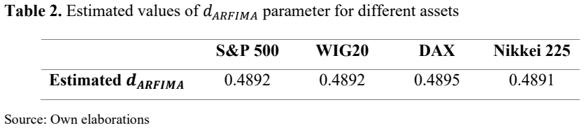
Minimum d for ADF stationarity, Section 3.2.1 Table 1.
d_ARFIMA (S&P 500) = 0.4892
Estimated from ARFIMA(0,d,0), Section 3.2.2 Table 2.
d_ARFIMA (WIG20) = 0.4892
Estimated from ARFIMA(0,d,0), Section 3.2.2 Table 2.
d_ARFIMA (DAX) = 0.4895
Estimated from ARFIMA(0,d,0), Section 3.2.2 Table 2.
d_ARFIMA (Nikkei 225) = 0.4891
Estimated from ARFIMA(0,d,0), Section 3.2.2 Table 2.
d_ARTFIMA (S&P 500) = 0.9895
Estimated from ARTFIMA(0,d,lambda,0), Section 3.2.2 Table 3.
lambda_ARTFIMA (S&P 500) = 0.0003
Estimated from ARTFIMA(0,d,lambda,0), Section 3.2.2 Table 3.
d_ARTFIMA (WIG20) = 1.0187
Estimated from ARTFIMA(0,d,lambda,0), Section 3.2.2 Table 3.
lambda_ARTFIMA (WIG20) = 0.0059
Estimated from ARTFIMA(0,d,lambda,0), Section 3.2.2 Table 3.
d_ARTFIMA (DAX) = 1.0050
Estimated from ARTFIMA(0,d,lambda,0), Section 3.2.2 Table 3.
lambda_ARTFIMA (DAX) = 0.0030
Estimated from ARTFIMA(0,d,lambda,0), Section 3.2.2 Table 3.
d_ARTFIMA (Nikkei 225) = 0.9953
Estimated from ARTFIMA(0,d,lambda,0), Section 3.2.2 Table 3.
lambda_ARTFIMA (Nikkei 225) = 0.0016
Estimated from ARTFIMA(0,d,lambda,0), Section 3.2.2 Table 3.
Fixed-width window threshold tau = not reported
Threshold in Eq. 24 for truncating fractional weights; never assigned a value, so implementation-dependent.

assumptions (4)

domain assumption The augmented Dickey-Fuller test at the 95% level is a valid criterion for choosing the minimal stationary differencing order.
Section 3.2.1 uses the ADF critical value -2.86 to set d_DePrado.
domain assumption ARFIMA(0,d,0) and ARTFIMA(0,d,lambda,0) provide reliable estimates of d and lambda for daily log index prices.
Section 3.2.2 uses the artfima R package; no goodness-of-fit diagnostics are reported.
ad hoc to paper Separate LSTM hyperparameter tuning per method does not confound the comparison of differencing methods.
Section 4.1 stages 7-8 tune different architectures for each asset and transformation, but architecture details are not reported.
domain assumption Inverse transformations from differentiated predictions to price levels are implemented correctly for all four methods.
Section 4.1 stage 10 states inverse operations are applied, but no code or formulas for the inversion are shown.

how reviews work

0 comments

Cite this review

Pith. "Pith review of Comparative analysis of financial data differentiation techniques using LSTM neural network." pith.science (2026). https://pith.science/paper/C533ZMV3

@misc{pith2026250519243,
  author       = {Pith},
  title        = {Pith review of: Comparative analysis of financial data differentiation techniques using LSTM neural network},
  year         = {2026},
  howpublished = {\url{https://pith.science/paper/C533ZMV3}},
  note         = {Machine review of arXiv:2505.19243}
}

read the original abstract

We compare traditional approach of computing logarithmic returns with the fractional differencing method and its tempered extension as methods of data preparation before their usage in advanced machine learning models. Differencing parameters are estimated using multiple techniques. The empirical investigation is conducted on data from four major stock indices covering the most recent 10-year period. The set of explanatory variables is additionally extended with technical indicators. The effectiveness of the differencing methods is evaluated using both forecast error metrics and risk-adjusted return trading performance metrics. The findings suggest that fractional differentiation methods provide a suitable data transformation technique, improving the predictive model forecasting performance. Furthermore, the generated predictions appeared to be effective in constructing profitable trading strategies for both individual assets and a portfolio of stock indices. These results underline the importance of appropriate data transformation techniques in financial time series forecasting, supporting the application of memory-preserving techniques.

Figures

Figures reproduced from arXiv: 2505.19243 by the authors.

**Figure 1.** Comparison of the weights for subsequent lagged observations for 𝑑 ∈ [0, 1] Source: Own elaborations based on De Prado (2018) [PITH_FULL_IMAGE:figures/full_fig_p021_1.png] view at source ↗

**Figure 2.** Comparison of the weights for subsequent lagged observations for 𝑑 ≥ 1 [PITH_FULL_IMAGE:figures/full_fig_p022_2.png] view at source ↗

**Figure 3.** Price levels of chosen market indices in years 2014-2023 Source: Own elaborations [PITH_FULL_IMAGE:figures/full_fig_p035_3.png] view at source ↗

Figures from the paper (9 more)

**Figure 5.** Figure 5: Comparison of ADF test statistic and Pearson coefficient of correlation for various values of fractional differencing parameter implemented for S&P 500 (USA) [PITH_FULL_IMAGE:figures/full_fig_p038_5.png]

**Figure 6.** Figure 6: Comparison of ADF test statistic and Pearson coefficient of correlation for various values of fractional differencing parameter implemented for WIG20 (Poland) Source: Own elaborations based on De Prado (2018) [PITH_FULL_IMAGE:figures/full_fig_p038_6.png]

**Figure 8.** Figure 8: Comparison of ADF test statistic and Pearson coefficient of correlation for various values of fractional differencing parameter implemented for Nikkei 225 (Japan) Source: Own elaborations based on De Prado (2018) [PITH_FULL_IMAGE:figures/full_fig_p039_8.png]

**Figure 9.** Figure 9: Comparison of original log-transformed series (black) and fractionally differenced series (grey) for different assets in years 2014-2023 [PITH_FULL_IMAGE:figures/full_fig_p041_9.png]

**Figure 10.** Figure 10: Comparison of original log-transformed series (black), fractionally differenced series (grey) and fractionally differenced series based on parameter estimated by ARFIMA model (blue) for different assets in years 2014-2023 Source: Own elaborations [PITH_FULL_IMAGE:fig…

**Figure 11.** Figure 11: Comparison of logarithmic returns series (black) and tempered-fractionally differenced series (blue) based on parameters estimated by ARTFIMA model for different assets in years 2014-2023 [PITH_FULL_IMAGE:figures/full_fig_p043_11.png]

**Figure 20.** Figure 20: Equity lines for 𝐿𝑜𝑛𝑔 − 𝑆ℎ𝑜𝑟𝑡 strategy, depending on different techniques of data differentiation for the portfolio of assets Equity lines represent a trading performance for different techniques of data differentiation in period from 01.01.2021 to 31.12.2023. Transac…

**Figure 21.** Figure 21: Equity lines for 𝐿𝑜𝑛𝑔 𝑂𝑛𝑙𝑦 strategy, depending on different techniques of data differentiation for the portfolio of assets Equity lines represent a trading performance for different techniques of data differentiation in period from 01.01.2021 to 31.12.2023. Transactio…

**Figure 12.** Figure 12: Equity lines for 𝐿𝑜𝑛𝑔 − 𝑆ℎ𝑜𝑟𝑡 strategy, depending on different techniques of data differentiation for S&P 500 Equity lines represent a trading performance for different techniques of data differentiation in period from 01.01.2021 to 31.12.2023. Transaction costs of 0.…

Discussion (0). Continue with ORCID to comment.

Reference graph

Works this paper leans on

21 extracted references · 21 canonical work pages

[1]

Akyildirim, E., Cepni, O., Corbet, S., & Uddin, G. S. (2023). Forecasting mid-price movement of Bitcoin futures using machine learning. Annals of Operations Research, 330(1), 553-584. Ammer, M. A., & Aldhyani, T. H. (2022). Deep learning algorithm to predict cryptocurrency fluctuation prices: Increasing investment awareness. Electronics, 11(15),

work page 2023
[2]

M., Sabzikar, F., & Chen, J

Meerschaert, M. M., Sabzikar, F., & Chen, J. (2015). Tempered fractional calculus. Journal of computational physics, 293,

work page 2015
[12]

Transaction costs of 0.005% are included (Kryńska and Ślepaczuk, 2022)

Equity lines for 𝐿𝑜𝑛𝑔−𝑆ℎ𝑜𝑟𝑡 strategy, depending on different techniques of data differentiation for S&P 500 Equity lines represent a trading performance for different techniques of data differentiation in period from 01.01.2021 to 31.12.2023. Transaction costs of 0.005% are included (Kryńska and Ślepaczuk, 2022). Source: Own elaborations 64 Indicator 𝚫𝑿𝒕 ...

work page 2021
[13]

M., & Latham, W

Dong, H., Bowers, H. M., & Latham, W. R. (2013). Evidence on the efficient market hypothesis from 44 global financial market indexes. Economics Research International, 2013(1), 238253. Erdas, M. L. (2019). Validity of weak-form market efficiency in Central and Eastern European countries (CEECs): Evidence from linear and nonlinear unit root tests. Review o...

work page 2013
[14]

M., Sabzikar, F., Phanikumar, M

Meerschaert, M. M., Sabzikar, F., Phanikumar, M. S., & Zeleke, A. (2014). Tempered fractional time series model for turbulence in geophysical flows. Journal of Statistical Mechanics: Theory and Experiment, 2014(9), P09023. Michańków, J., Sakowski, P., & Ślepaczuk, R. (2022). LSTM in algorithmic investment strategies on BTC and S&P500 index. Sensors, 22(3),

work page 2014
[15]

Transaction costs of 0.005% are included (Kryńska and Ślepaczuk, 2022)

Equity lines for 𝐿𝑜𝑛𝑔 𝑂𝑛𝑙𝑦 strategy, depending on different techniques of data differentiation for S&P 500 Equity lines represent a trading performance for different techniques of data differentiation in period from 01.01.2021 to 31.12.2023. Transaction costs of 0.005% are included (Kryńska and Ślepaczuk, 2022). Source: Own elaborations 65 Indicator 𝚫𝑿𝒕 𝜟...

work page 2021
[16]

Transaction costs of 0.005% are included (Kryńska and Ślepaczuk, 2022)

Equity lines for 𝐿𝑜𝑛𝑔−𝑆ℎ𝑜𝑟𝑡 strategy, depending on different techniques of data differentiation for WIG20 Equity lines represent a trading performance for different techniques of data differentiation in period from 01.01.2021 to 31.12.2023. Transaction costs of 0.005% are included (Kryńska and Ślepaczuk, 2022). Source: Own elaborations 66 Indicator 𝚫𝑿𝒕 𝜟𝒅...

work page 2021
[17]

Transaction costs of 0.005% are included (Kryńska and Ślepaczuk, 2022)

Equity lines for 𝐿𝑜𝑛𝑔 𝑂𝑛𝑙𝑦 strategy, depending on different techniques of data differentiation for WIG20 Equity lines represent a trading performance for different techniques of data differentiation in period from 01.01.2021 to 31.12.2023. Transaction costs of 0.005% are included (Kryńska and Ślepaczuk, 2022). Source: Own elaborations 67 Indicator 𝚫𝑿𝒕 𝜟𝒅𝑫...

work page 2021

Show all 21 references

[18]

Transaction costs of 0.005% are included (Kryńska and Ślepaczuk, 2022)

Equity lines for 𝐿𝑜𝑛𝑔−𝑆ℎ𝑜𝑟𝑡 strategy, depending on different techniques of data differentiation for DAX Equity lines represent a trading performance for different techniques of data differentiation in period from 01.01.2021 to 31.12.2023. Transaction costs of 0.005% are includ...

2021
[19]

Transaction costs of 0.005% are included (Kryńska and Ślepaczuk, 2022)

Equity lines for 𝐿𝑜𝑛𝑔 𝑂𝑛𝑙𝑦 strategy, depending on different techniques of data differentiation for DAX Equity lines represent a trading performance for different techniques of data differentiation in period from 01.01.2021 to 31.12.2023. Transaction costs of 0.005% are include...

2021
[20]

Transaction costs of 0.005% are included (Kryńska and Ślepaczuk, 2022)

Equity lines for 𝐿𝑜𝑛𝑔−𝑆ℎ𝑜𝑟𝑡 strategy, depending on different techniques of data differentiation for Nikkei 225 Equity lines represent a trading performance for different techniques of data differentiation in period from 01.01.2021 to 31.12.2023. Transaction costs of 0.005% are...

2021
[21]

Transaction costs of 0.005% are included (Kryńska and Ślepaczuk, 2022)

Equity lines for 𝐿𝑜𝑛𝑔 𝑂𝑛𝑙𝑦 strategy, depending on different techniques of data differentiation for Nikkei 225 Equity lines represent a trading performance for different techniques of data differentiation in period from 01.01.2021 to 31.12.2023. Transaction costs of 0.005% are ...

2021
[26]

(2021, January)

Shobana, G., & Umamaheswari, K. (2021, January). Forecasting by machine learning techniques and econometrics: A review. In 2021 6th international conference on inventive computation technologies (ICICT) (pp. 1010-1016). IEEE. Sze, V., Chen, Y. H., Yang, T. J., & Emer, J. S. (2...

2017
[50]

Harvey, A. C. (1990). Forecasting, structural time series models and the Kalman filter. Hochreiter, S. (1998). The vanishing gradient problem during learning recurrent neural nets and problem solutions. International Journal of Uncertainty, Fuzziness and Knowledge-Based System...

1990
[84]

Naseer, M., & Bin Tariq, D. Y. (2015). The efficient market hypothesis: A critical review of the literature. The IUP journal of financial risk management, 12(4), 48-63. Nelson, D. M., Pereira, A. C., & De Oliveira, R. A. (2017, May). Stock market's price movement prediction wi...

2015
[117]

Sewell, M. (2012). The efficient market hypothesis: Empirical evidence. International Journal of Statistics and Probability, 1(2), 164-178. Shah, D., Isah, H., & Zulkernine, F. (2019). Stock market analysis: A review and taxonomy of prediction techniques. International Journal...

2012
[158]

Yajima, Y. (1985). On estimation of long‐memory time series models. Australian Journal of Statistics, 27(3), 303-320. Yang, C., Zhai, J., & Tao, G. (2020). Deep learning for price movement prediction using convolutional neural network and long short‐term memory. Mathematical P...

1985 arXiv
[687]

Kabala, J., & Sabzikar, F. (2021). Statistical inference for ARTFIMA time series with stable innovations. arXiv preprint arXiv:2103.07717. Kashif, K., & Ślepaczuk, R. (2025). LSTM-ARIMA as a hybrid approach in algorithmic investment strategies. Knowledge-Based Systems. Kidd, D...

2021 arXiv
[917]

Michańków, J., Sakowski, P., & Ślepaczuk, R. (2024). Mean Absolute Directional Loss as a new loss function for machine learning problems in algorithmic investment strategies. Journal of Computational Science, 81, 102375. Mirete-Ferrer, P. M., Garcia-Garcia, A., Baixauli-Soler,...

2024
[2349]

A., Adewumi, A

Ariyo, A. A., Adewumi, A. O., & Ayo, C. K. (2014, March). Stock price prediction using the ARIMA model. In 2014 UKSim-AMSS 16th international conference on computer modelling and simulation (pp. 106-112). IEEE. Assaf, A. (2006). Dependence and mean reversion in stock prices: T...

2006 arXiv
[2717]

Ryś, P., & Ślepaczuk, R. (2019). Machine Learning Methods in Algorithmic Trading Strategy Optimization–Design and Time Efficiency. Central European Economic Journal, 5(52). Sabzikar, F., Kabala, J., & Burnecki, K. (2022). Tempered fractionally integrated process with stable no...

2019

Pith tools

Reviewed August 7, 2026 · model on record in the stance chip above.

[1] [1]

Akyildirim, E., Cepni, O., Corbet, S., & Uddin, G. S. (2023). Forecasting mid-price movement of Bitcoin futures using machine learning. Annals of Operations Research, 330(1), 553-584. Ammer, M. A., & Aldhyani, T. H. (2022). Deep learning algorithm to predict cryptocurrency fluctuation prices: Increasing investment awareness. Electronics, 11(15),

work page 2023

[2] [2]

M., Sabzikar, F., & Chen, J

Meerschaert, M. M., Sabzikar, F., & Chen, J. (2015). Tempered fractional calculus. Journal of computational physics, 293,

work page 2015

[3] [12]

Transaction costs of 0.005% are included (Kryńska and Ślepaczuk, 2022)

Equity lines for 𝐿𝑜𝑛𝑔−𝑆ℎ𝑜𝑟𝑡 strategy, depending on different techniques of data differentiation for S&P 500 Equity lines represent a trading performance for different techniques of data differentiation in period from 01.01.2021 to 31.12.2023. Transaction costs of 0.005% are included (Kryńska and Ślepaczuk, 2022). Source: Own elaborations 64 Indicator 𝚫𝑿𝒕 ...

work page 2021

[4] [13]

M., & Latham, W

Dong, H., Bowers, H. M., & Latham, W. R. (2013). Evidence on the efficient market hypothesis from 44 global financial market indexes. Economics Research International, 2013(1), 238253. Erdas, M. L. (2019). Validity of weak-form market efficiency in Central and Eastern European countries (CEECs): Evidence from linear and nonlinear unit root tests. Review o...

work page 2013

[5] [14]

M., Sabzikar, F., Phanikumar, M

Meerschaert, M. M., Sabzikar, F., Phanikumar, M. S., & Zeleke, A. (2014). Tempered fractional time series model for turbulence in geophysical flows. Journal of Statistical Mechanics: Theory and Experiment, 2014(9), P09023. Michańków, J., Sakowski, P., & Ślepaczuk, R. (2022). LSTM in algorithmic investment strategies on BTC and S&P500 index. Sensors, 22(3),

work page 2014

[6] [15]

Transaction costs of 0.005% are included (Kryńska and Ślepaczuk, 2022)

Equity lines for 𝐿𝑜𝑛𝑔 𝑂𝑛𝑙𝑦 strategy, depending on different techniques of data differentiation for S&P 500 Equity lines represent a trading performance for different techniques of data differentiation in period from 01.01.2021 to 31.12.2023. Transaction costs of 0.005% are included (Kryńska and Ślepaczuk, 2022). Source: Own elaborations 65 Indicator 𝚫𝑿𝒕 𝜟...

work page 2021

[7] [16]

Transaction costs of 0.005% are included (Kryńska and Ślepaczuk, 2022)

Equity lines for 𝐿𝑜𝑛𝑔−𝑆ℎ𝑜𝑟𝑡 strategy, depending on different techniques of data differentiation for WIG20 Equity lines represent a trading performance for different techniques of data differentiation in period from 01.01.2021 to 31.12.2023. Transaction costs of 0.005% are included (Kryńska and Ślepaczuk, 2022). Source: Own elaborations 66 Indicator 𝚫𝑿𝒕 𝜟𝒅...

work page 2021

[8] [17]

Transaction costs of 0.005% are included (Kryńska and Ślepaczuk, 2022)

Equity lines for 𝐿𝑜𝑛𝑔 𝑂𝑛𝑙𝑦 strategy, depending on different techniques of data differentiation for WIG20 Equity lines represent a trading performance for different techniques of data differentiation in period from 01.01.2021 to 31.12.2023. Transaction costs of 0.005% are included (Kryńska and Ślepaczuk, 2022). Source: Own elaborations 67 Indicator 𝚫𝑿𝒕 𝜟𝒅𝑫...

work page 2021