Fast-Decaying Polynomial Reproduction

Giacomo Cappellazzo; Stefano De Marchi

REVIEW 3 major objections 5 minor 2 references

Fast-Decaying Polynomial Reproduction

T0 review · 3 major / 5 minor · reviewed 2026-08-12 · deepseek-v4-flash

Challenge this review Re-run · record.json Download PDF Read on arXiv ↗ Review JSON

Pith's one-line read Replacing compactly supported basis functions by fast-decaying ones still yields stable quasi-interpolants that reproduce polynomials and converge at order $O(h^{m+1})$ on quasi-uniform node sets.

desk verdict Fast-decaying polynomial reproduction is a worthwhile generalization; Theorem 2's constant has a repairable flaw, and the ℓ1 scheme is a genuinely new contribution. read the letter →

arxiv 2411.14933 v1 pith:C7MSEENO submitted 2024-11-22 math.NA cs.NA

Stefano De Marchi , Giacomo Cappellazzo This is my paper · ORCID

classification math.NAcs.NA MSC 41A0541A1041A2565D0565D15

keywords polynomialreproductionfast-decayingbasisfunctionsquasi-interpolationmovingleastsquareslinearprogrammingapproximationLebesgueconstantscattereddataconvergencerates

verification ladder T0 review T1 audit T2 compute T3 formal

The pith

A machine-rendered reading of the paper's core claim, the machinery that carries it, and where it could break.

The reading

Local polynomial reproduction usually demands compactly supported basis functions, and that excludes useful global kernels such as the rescaled localized radial basis functions. The paper proposes a relaxation: instead of vanishing outside a fixed ball, each basis function only has to decay fast relative to the separation distance of the node set. With that single change, quasi-interpolants that reproduce polynomials of degree $m$ are shown to be stable and to converge at rate $O(h^{m+1})$ on quasi-uniform data. The framework is instantiated on Gaussian moving least squares and on an $\ell^1$ linear-programming scheme, both with explicitly derived decay envelopes, and the paper reports numerical confirmation in one and two dimensions.

What carries the argument

The machinery is the decay envelope plus an annulus-counting estimate. Definition 4 requires each basis function to be bounded by $C \varphi(\|x-x_j\|/q_X)$, where $\varphi$ has the geometric-decay ratio condition $\lim_{n\to\infty} \varphi(n+1)/\varphi(n) < 1$. Theorem 2 partitions the domain into annuli $\{n q_X \le \|x-x_j\| \le (n+1)q_X\}$, counts at most $3^d (n+1)^{d-1}$ nodes in each annulus, and sums the weighted decay; the geometric ratio condition makes the series $K = 3^d C \sum_{n=0}^\infty (n+1)^{d+\ell-1}\varphi(n)$ converge. That weighted-moment estimate is the input to a Taylor-expansion proof in Theorem 3. For the two instantiations, the local polynomial reproduction theorem supplies an admissible competitor in the moving least squares or linear-programming optimization problem, which forces the optimized basis functions to inherit a Gaussian or exponential envelope with constants $C$ and $\varphi$ stated explicitly in (12) through (17).

What would settle it

Take a fixed quasi-uniform sequence of nodes in three dimensions, set polynomial degree $m=5$ with a Gaussian weight, compute the basis functions from the moving least squares system, and measure the left-hand side of the decay bound (12) as the fill distance shrinks; if that quantity grows without bound, or if the $L_\infty$ error against a $C^6$ test function does not track $h^6$ once $h$ falls below the stated threshold, then the convergence claim of the paper is false.

Watch

Extended reading notes

Core claim

The paper's central claim is that the essential content of local polynomial reproduction is not compact support but controlled decay: Definition 4 asks for $|u_j(x)| \le C \varphi(\|x-x_j\|/q_X)$ with $\varphi$ decaying faster than any geometric progression. Under this condition, Theorem 2 bounds every weighted moment sum $\sum_j \|x-x_j\|^\ell |u_j(x)|$ by a constant times $q_X^\ell$, which gives a uniform stability estimate, and Theorem 3 converts that into the optimal algebraic error bound $K h_{X,\Omega}^{m+1}\|f\|_{C^{m+1}(\Omega^*)}$ for $C^{m+1}$ functions. The two concrete methods, Gaussian moving least squares and the $\ell^1$ linear program, are proved to satisfy Definition 4 by using a classical local polynomial reproduction basis as a feasible comparison point, yielding explicit exponential envelopes. This recovers and extends the RL-RBF convergence analysis and puts smooth global-kernel quasi-interpolants on the same footing as compactly supported ones.

Load-bearing premise

The load-bearing premise is that the classical local polynomial-reproduction basis used to seed the proofs exists with constants that do not grow destructively as the target polynomial degree or the dimension grows; if they do, the fast decay rates derived become too weak to guarantee the advertised convergence.

Editorial extensions

If this is right

Any method whose basis functions satisfy the decay condition of Definition 4 automatically has uniformly bounded Lebesgue constants and the same optimal order $h^{m+1}$ error, independent of how the basis functions are constructed.
Gaussian moving least squares gives a $C^\infty$ approximant that converges at the optimal rate, addressing the usual non-convergence of fixed-parameter Gaussian approximate-approximation schemes by tying the scale $\delta$ to the data distribution.
The $\ell^1$ scheme produces vertex solutions of a linear program, so at each evaluation point at most $Q = \dim \pi_m(\mathbb{R}^d)$ basis functions are nonzero; evaluation costs $O(N)$ to build and $O(Q)$ to apply.
The framework includes algebraic-decay kernels as a degenerate limit, with explicit thresholds on the decay exponent needed for stability and convergence.
The RL-RBF method is subsumed as a special case, so its convergence proof can be read through Definition 4 rather than through compact support.

Reading between the lines

Editorial extensions of the paper, not claims the author makes directly.

Beyond the paper, one could test kernels outside the two examples, such as Matérn or inverse multiquadric functions, by checking whether their tails satisfy the Definition 4 ratio condition; the same theorems would then give rates and stability without new proofs.
The explicit constant $K$ in (5) suggests a concrete optimization problem: among admissible envelopes $\varphi$ with a fixed budget for the Lebesgue constant, choose the one minimizing the error constant.
The $\ell^1$ scheme's sparse vertex representation at each point hints at a connection to compressed sensing: on random node sets one could ask whether the polynomial-reproducing subset selected by the simplex method is unique and stable under noise.
For algebraic decay, the paper's threshold conditions imply a sharp stability phase transition in the exponent $k$; a systematic numerical scan across $k$ and dimension $d$ would map where the method switches from convergent to divergent.

Share X Bluesky LinkedIn Reddit HN

Editorial analysis

A structured set of objections, weighed in public.

Desk editor's note, referee report, and a circularity audit.

Desk Editor's Note

read the letter

Briefly: the paper deserves a serious referee, but it needs a revision before the results are citable as printed. The core idea — replace compact support in local polynomial reproduction with fast decay relative to the separation radius — is a genuine generalization, and the two instantiations, Gaussian moving least squares and an ℓ1 linear-programming scheme, are worked out with explicit constants. Theorems 4 and 5 correctly adapt Wendland's local polynomial reproduction theorem, and Theorem 3's convergence statement follows cleanly from the weighted-sum bound in Theorem 2. The ℓ1 scheme is the most interesting part: the simplex vertex solution gives at most Q nonzero basis functions per evaluation point, which is a real computational benefit and a new application of sparse optimization in this setting.

Now the soft spots. The proof of Theorem 2 contains a false inequality. The volume comparison gives #{xj ∈ E_n} ≤ (n+2)^d − (n−1)^d, but the next bound, ≤ 3d n^{d−1}, is not true — it already fails for d=5, n=1 (243 > 15). The stated constant K in (5) is therefore unsupported. The fix is local: a mean-value argument gives ≤ 3d(n+2)^{d−1}, and the series still converges because φ decays at least geometrically. So the stability and convergence results survive with a larger d-dependent constant, but the proof as printed has a hole.

The abstract also overclaims the numerics: the ℓ1 experiments demonstrate sparsity (at most Q nonzero coefficients per evaluation), not compact support of the basis functions. The numerical section has other v1 issues — no code or data shipped, δ set by trial and error, and some figure/text mismatches in axes and domains. These are presentation problems, not mathematical ones. The citation pattern is fine; the self-citation to [DW20] is appropriate, and Wendland's external theorem is the standard anchor.

Verdict: central framework and applications are sound in spirit and mostly in detail, but Theorem 2's constant needs repair. I would send this to a competent referee rather than desk-reject; with a short revision it could become a solid paper for the approximation-theory audience.

Referee Report

3 major / 5 minor

Summary. The manuscript proposes a relaxation of local polynomial reproduction in which the compact-support condition of Definition 1 is replaced by a fast-decay condition for the basis functions (Definition 4). The main theoretical results are: Theorem 2, a bound on the weighted sums \sum_j \|x-x_j\|^\ell |u_j(x)| by K q_X^\ell; Theorem 3, an O(h_{X,\Omega}^{m+1}) convergence estimate for quasi-interpolants that reproduce \pi_m(R^d); Theorem 4, verifying the framework for Gaussian moving-least-squares weights; and Theorem 5, verifying it for an \ell_1-minimization scheme. Numerical experiments in Section 6 illustrate smoothness, sparsity, Lebesgue constants, and convergence rates, including multivariate tests.

Significance. If the proof gaps are repaired, the paper offers a genuinely useful framework: it generalizes Wendland's local polynomial reproduction to non-compactly supported basis functions, provides explicit decay functions and constants for Gaussian MLS and \ell_1 quasi-interpolation, and connects the RL-RBF method to a broader theory. The proofs are constructive and the convergence and stability statements are quantitative, which is a valuable feature. The numerical experiments support the main convergence and stability claims, although they do not establish compact support of the \ell_1 basis functions.

major comments (3)

[Section 3.1, proof of Theorem 2 and Eq. (5)] The volume-counting inequality used to define the constant K is false as stated. The proof asserts \#\{x_j: x_j \in E_n\} \le (n+2)^d - (n-1)^d \le 3d(n+1)^{d-1}, but for n=1 and d=5 the rightmost inequality reads 3^5 \le 15 \cdot 2^4, i.e. 243 \le 240, which fails. The sentence 'The above inequalities are held by induction on d' is not a proof and is contradicted by this counterexample. The gap is local and repairable: a mean-value estimate gives (n+2)^d - (n-1)^d \le 3d\,2^{d-1}(n+1)^{d-1}, so the same stability and convergence conclusions follow with a larger d-dependent constant. As printed, however, the constant K in Eq. (5), and therefore the Lebesgue-constant bound and the error constant in Theorem 3, are not justified.
[Section 5, proof of Theorem 5] There is a sign error in the Gaussian-weight case. From the preceding bound \sum_i |\tilde u_i(x)| / w_i(x) \le C_1 e^{\nu(C_2 h_{X,\Omega}/\delta)^2}, each coefficient must inherit the positive exponent, so the displayed inequality should contain e^{+\nu(C_2/(\gamma c_\gamma))^2}, not e^{-\nu(C_2/(\gamma c_\gamma))^2}. As printed, the constant C = e C_1 e^{-\nu(C_2/(\gamma c_\gamma))^2} is too small and the upper bound is not derived from the preceding step. This is a load-bearing error in one of the two central instantiations, but it is easily fixed by changing the sign of that exponent, yielding C = e C_1 e^{+\nu(C_2/(\gamma c_\gamma))^2}.
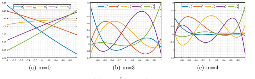
[Abstract and Section 6.1] The abstract states that compactness of the support has been verified numerically, but the experiments do not verify compact support. For the \ell_1 scheme, the simplex-method argument only shows that at each evaluation point at most Q coefficients in the representation are nonzero (a vertex solution), i.e. sparsity of the representation; Figures 3, 4, and 6 illustrate basis functions over a finite grid and cannot establish that each a_j^*(x) has compact support. The overclaim should be removed or replaced by a statement about sparsity.

minor comments (5)

[Section 4, Eq. (7)] The notation a^T D(x) a with D diagonal of entries e^{-\nu(\|x-x_i\|/\delta)^2} is inconsistent with the displayed minimization \sum_i a_i(x)^2 / e^{-\nu(\|x-x_i\|/\delta)^2}; the quadratic form should use D(x)^{-1} or the definition of D should be changed accordingly.
[Section 4, Eq. (9)] The symbol 'QX' in the displayed expression for a_j^*(x) appears to be a typesetting artifact; it should read \sum_{k=1}^Q.
[Section 6.2, Figures 7 and 8] The text describes the domain for Franke's function as [0,1]^2, but the figure captions state \|f-z_{f,X}\|_{L_\infty([-1,1])}; the domain and the x-axis labeling ('25 to 30' versus node counts 676-961) need to be reconciled.
[Section 6.1] The phrase 'only m+1 basis functions are different from zero' should be qualified as 'at each evaluation point for a vertex solution of the linear program'; without this qualification it could be misread as a statement of compact support.
[Theorems 4 and 5] The paper would benefit from an explicit remark that the constants C and h_0 in Theorems 4 and 5 inherit the dependence on m, d, and the cone parameters through the constants C_1 and C_2 of Theorem 1, so the practical convergence statement may require very small fill distances for large m or d.

Circularity Check

0 steps flagged · score 0.0 of 10

No significant circularity: the stability and convergence claims follow from the explicit decay/reproduction definition and Wendland's external polynomial-reproduction theorem, with no fitted parameter or author-supplied uniqueness result carrying the argument.

full rationale

The derivation chain is definition-driven rather than circular. Definition 4 explicitly assumes exact polynomial reproduction plus a per-node decay bound, and Theorem 2 derives the moment inequality (4) from that definition by a direct volume-counting argument; Theorem 3 then derives the O(h^{m+1}) error bound by Taylor expansion together with the same moment inequality. Neither conclusion is quietly assumed in the input. Theorems 4 and 5 use Wendland's local polynomial reproduction theorem ([Wen04, Theorem 3.14]) as an independent external ingredient to bound the moving-least-squares or linear-programming objective, and then derive the decay functions explicitly in (12)-(14) and (16)-(17); no parameter is fitted to force the theorems, and the constants C and phi are given in closed form. The self-references to [DW20] (the delta-scaling convention and the label 'straightforward generalization' in Theorem 2) and to [Cap22] (one-dimensional numerical context) are motivational or contextual; the paper supplies its own proofs, so these citations are not load-bearing. Two non-circular issues should nevertheless be flagged explicitly. First, the proof of Theorem 2 contains an unsupported, and as printed false for d=5, volume-count inequality ((n+2)^d - (n-1)^d <= 3d(n+1)^{d-1}), so the stated constant K in (5) is not justified as written; a larger d-dependent constant repairs the convergence conclusion, so this is a correctness gap rather than a circularity. Second, the abstract's claim that 'compactness of the support' was verified numerically is not supported by the experiments, which demonstrate only that each evaluation uses at most m+1 nonzero coefficients under the simplex method (sparsity), not compact support of basis functions. Neither issue affects the circularity verdict.

Assumptions & free parameters 3 free parameters · 4 assumptions · 0 invented entities

The central theorems draw on Wendland's external local polynomial reproduction theorem, on standard quasi-uniformity and unisolvence assumptions, and on the new decay-ratio hypothesis that defines the framework. The numerical parameters δ, ν, and k are hand-chosen inputs to the experiments, not fitted quantities used to prove the theorems.

free parameters (3)

δ (weight scaling) = δ = 5h (univariate and stability) and δ = 30h (2D convergence, chosen by trial and error)
The Gaussian weight depends on δ; the theory requires γcγh ≤ δ ≤ cγh, and the numerical tests choose specific values, with the 2D value reported as trial-and-error.
ν (Gaussian exponent) = ν = 1 (implied by w = e^{-(|x−y|/δ)^2})
The Gaussian weight parameter in Theorems 4-5 and all experiments; a generic positive constant in the theory.
k (algebraic decay exponent) = k = 6.2 and k = 3.1 in Figure 9
Chosen to satisfy the derived constraints d+m−k/2<−1 (MLS) and d+m−k<−1 (ℓ1) in the degenerate algebraic-decay tests.

assumptions (4)

standard math Existence of a local polynomial reproduction basis with support radius C2 h and L1-sum ≤ C1 for every quasi-uniform X with h ≤ h0 (Wendland 2004, Theorem 3.14, stated as Theorem 1).
Invoked in the proofs of Theorems 4 and 5 to produce a feasible comparison basis for the MLS and LP minimizations.
domain assumption Ω satisfies an interior cone condition and X is quasi-uniform, with q_X ≤ h_{X,Ω} ≤ cqu q_X.
Definitions 2 and 3; used throughout to relate separation and fill distances and to apply Theorem 1.
domain assumption The node set X is π_m(R^d)-unisolvent, making the MLS and LP minimizers unique.
Stated before equation (6) and used to define a^* in (7)-(9) and (15).
ad hoc to paper The decay function φ in Definition 4 is decreasing and satisfies lim_{n→∞} φ(n+1)/φ(n) < 1.
This ratio-test condition is the defining hypothesis of the new fast-decaying framework; it ensures the constant K in Theorem 2 is finite.

how reviews work

0 comments

Cite this review

Pith. "Pith review of Fast-Decaying Polynomial Reproduction." pith.science (2026). https://pith.science/paper/C7MSEENO

@misc{pith2026241114933,
  author       = {Pith},
  title        = {Pith review of: Fast-Decaying Polynomial Reproduction},
  year         = {2026},
  howpublished = {\url{https://pith.science/paper/C7MSEENO}},
  note         = {Machine review of arXiv:2411.14933}
}

read the original abstract

Polynomial reproduction plays a relevant role in deriving error estimates for various approximation schemes. Local reproduction in a quasi-uniform setting is a significant factor in the estimation of error and the assessment of stability but for some computationally relevant schemes, such as Rescaled Localized Radial Basis Functions (RL-RBF), it becomes a limitation. To facilitate the study of a greater variety of approximation methods in a unified and efficient manner, this work proposes a framework based on fast decaying polynomial reproduction: we do not restrict to compactly supported basis functions, but we allow the basis function decay to infinity as a function of the separation distance. Implementing fast decaying polynomial reproduction provides stable and convergent methods, that can be smooth when approximating by moving least squares otherwise very efficient in the case of linear programming problems. All the results presented in this paper concerning the rate of convergence, the Lebesgue constant, the smoothness of the approximant, and the compactness of the support have been verified numerically, even in the multivariate setting.

Figures

Figures reproduced from arXiv: 2411.14933 by the authors.

**Figure 1.** The weight function w(x) = e −x 2 ∈ C∞(R), the nodes are 5 uniformly perturbed equispaced nodes in [−1, 1]. From left to right the basis functions reproduce the polynomials of degrees m = 0, 3, and 4 respectively. In this numerical test δ = 5hX,Ω. functions does not affect the convergence rate but a smooth approximant can be useful in applications. To produce [PITH_FULL_IMAGE:figures/full_fig_p018_1.png] view at source ↗

**Figure 2.** Basis functions of Theorem 4. The weight function coincides with [PITH_FULL_IMAGE:figures/full_fig_p018_2.png] view at source ↗

**Figure 3.** Basis functions of equation (15). The weight function coincides with [PITH_FULL_IMAGE:figures/full_fig_p019_3.png] view at source ↗

Figures from the paper (7 more)

**Figure 4.** Figure 4: Basis functions of equation (15). The weight function coincides with [PITH_FULL_IMAGE:figures/full_fig_p019_4.png]

**Figure 5.** Figure 5: Basis functions of Theorem 4. The weight function coincides with [PITH_FULL_IMAGE:figures/full_fig_p020_5.png]

**Figure 6.** Figure 6: Basis functions of equation (15). The weight function coincides with [PITH_FULL_IMAGE:figures/full_fig_p021_6.png]

**Figure 7.** Figure 7: Convergence rate of the approximation error [PITH_FULL_IMAGE:figures/full_fig_p022_7.png]

**Figure 8.** Figure 8: Convergence rate of the approximation error [PITH_FULL_IMAGE:figures/full_fig_p023_8.png]

**Figure 9.** Figure 9: Convergence rate of the approximation error [PITH_FULL_IMAGE:figures/full_fig_p024_9.png]

**Figure 10.** Figure 10: Lebesgue constants of the methods in equation (6) and in equation (15) re [PITH_FULL_IMAGE:figures/full_fig_p025_10.png]

Discussion (0). Continue with ORCID to comment.

Reference graph

Works this paper leans on

2 extracted references

[300]

[Wen04] Holger Wendland

url: https://api.semanticscholar.org/CorpusID:120212734. [Wen04] Holger Wendland. Scattered Data Approximation . Cambridge Monographs on Applied and Computational Mathematics. Cambridge University Press, 2004. doi: 10.1017/CBO9780511617539. 29

doi:10.1017/cbo9780511617539 2004
[2008]

Surfaces generated by moving least squares methods

isbn: 9780817648435. url: https : / / books . google . it / books ? id = Sld1YYAedtgC. [LS81] Peter Lancaster and Kestutis Salkauskas. “Surfaces generated by moving least squares methods”. In: Mathematics of Computation 37 (1981), pp. 141–158. [LC92] W.A. Light and E.W. Cheney. “Quasi-interpolation with translates of a function having noncompact support”....

arXiv 1981

Pith tools

Reviewed August 12, 2026 · model on record in the stance chip above.

[1] [300]

[Wen04] Holger Wendland

url: https://api.semanticscholar.org/CorpusID:120212734. [Wen04] Holger Wendland. Scattered Data Approximation . Cambridge Monographs on Applied and Computational Mathematics. Cambridge University Press, 2004. doi: 10.1017/CBO9780511617539. 29

doi:10.1017/cbo9780511617539 2004

[2] [2008]

Surfaces generated by moving least squares methods

isbn: 9780817648435. url: https : / / books . google . it / books ? id = Sld1YYAedtgC. [LS81] Peter Lancaster and Kestutis Salkauskas. “Surfaces generated by moving least squares methods”. In: Mathematics of Computation 37 (1981), pp. 141–158. [LC92] W.A. Light and E.W. Cheney. “Quasi-interpolation with translates of a function having noncompact support”....

arXiv 1981