REVIEW 3 major objections 5 minor 69 references
Synthetic supply networks
T0 review · 3 major / 5 minor · reviewed 2026-08-15 · deepseek-v4-flash
Pith's one-line read A public-data method generates synthetic firm-level supply networks that match both micro statistics and national input-output tables.
desk verdict Useful and well-engineered pipeline, but the abstract overclaims: the match is to a selected set of moments, not all known network properties. read the letter →
The pith
A machine-rendered reading of the paper's core claim, the machinery that carries it, and where it could break.
The reading
What carries the argument
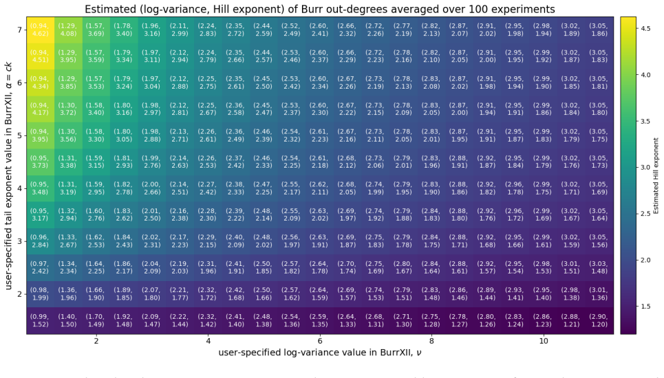
The load-bearing objects are the Burr XII distribution—a three-parameter heavy-tailed distribution whose asymptotic tail exponent is the product of two parameters, used to draw in- and out-degree sequences—and the gravity-like weight formula that combines node degrees with lognormal 'fitness' latent variables. Sampling degrees separately and then reordering one sequence with rank-dependent lognormal noise induces the empirical in-out degree correlation of about 0.55 while preserving marginals. The configuration model turns the degree sequences into a binary directed graph; the weight formula then assigns positive values to existing edges; and the rescaling identity $W_{ij} = W^{\mathrm{init}}_{ij} \cdot \mathrm{IOT}_{g_i g_j} / \sum_{f \in g_i, h \in g_j} W^{\mathrm{init}}_{fh}$ guarantees the industry-level sums equal the target table. The final mechanism is the calibration loop, which searches over the four exponents to match the targeted weighted-network statistics.
What would settle it
Take a country whose full firm-to-firm VAT network is known but not yet published, generate a synthetic network using only the public input-output table and the stated targets, then compare the two networks on untargeted statistics—reciprocity, clustering, assortativity, and sectoral concentration; if the observed real values fall far outside the synthetic distributions, the claim that public data suffice to reproduce plausible firm-level structure is refuted.
Extended reading notes
Core claim
The central claim is that a directed, weighted firm-level production network can be generated in four stages—Burr XII degree sampling, degree-sequence coupling, configuration-model wiring, and weight assignment with input-output rescaling—so that the final object matches a chosen set of firm-level statistics while its industry-level aggregation equals a given input-output table exactly. The weight assignment uses a gravity-like formula on node degrees and latent fitnesses, $W^{\mathrm{init}}_{ij} = (f^{\mathrm{out}}_i)^{\theta_{f,\mathrm{out}}} (f^{\mathrm{in}}_j)^{\theta_{f,\mathrm{in}}} (k^{\mathrm{out}}_i)^{\theta_{k,\mathrm{out}}} (k^{\mathrm{in}}_j)^{\theta_{k,\mathrm{in}}} A_{ij}$, and the rescaling step multiplies each edge weight by the ratio of the target industry-pair flow to the current aggregated flow, which guarantees exact agreement at the industry level. A calibration loop adjusts the four exponents to minimize squared discrepancies between synthetic and empirical tail exponents, correlations, regression slopes, and log-variances. The paper reports that the calibrated network matches the targeted micro moments, reproduces plausible univariate and joint distributions, and remains stable across network sizes from 10,000 to 500,000 firms and across different countries' input-output tables.
Load-bearing premise
The load-bearing premise is that the empirical statistics taken from the survey of firm-level networks are the right and sufficient summary of a real production network, and that input-output tables and VAT-based transaction data are compatible enough that rescaling to industry totals does not distort the micro properties.
Editorial extensions
If this is right
- Researchers can generate a plausible firm-level supply network for any country with a published input-output table, using only public data, so confidential administrative records are not needed.
- Macroeconomic and agent-based models can be initialized at a one-to-one scale with realistic firm heterogeneity, enabling stress tests and shock propagation studies that previously required private transaction data.
- Because the rescaled network aggregates exactly to the input-output table, model outcomes remain consistent with national accounting aggregates by construction.
- The same calibrated weight parameters can be reused across countries and network sizes without re-running the optimization, making the pipeline cheap to deploy.
- The method scales roughly linearly with the number of firms, up to 500,000 firms, so it remains tractable for large-scale economic models.
Reading between the lines
- The same pipeline could plausibly be extended to worker–firm and household–firm bipartite networks once public moments from administrative or scanner data become available; the paper only gestures at this possibility.
- Because the method relies on a small set of cross-country moments, a strongly non-universal country would receive a plausible-looking but wrong network that still passes all stated targets; this is an inference from the paper's reliance on the survey statistics.
- Since the configuration-model step yields lower reciprocity and clustering than real networks, downstream applications sensitive to local triadic structure may need a topology-preserving extension; the paper notes the limitation but does not address it.
- A direct stress test would compare crisis simulations on synthetic versus observed networks in countries with VAT data, a comparison the paper suggests but leaves to future work.
Signed reviews
Editorial analysis
A structured set of objections, weighed in public.
Referee Report
Summary. The paper introduces a method for generating synthetic firm-level supply networks from publicly available data. The pipeline has four stages: sampling in- and out-degree sequences from calibrated Burr XII distributions, reordering them to induce the empirical in-out degree correlation, drawing a binary network from the configuration model, and then assigning weights via a gravity-like formula involving firm fitnesses and degrees, followed by industry assignment and rescaling so that the aggregate matches a target OECD input-output table. The four weight exponents are calibrated by Optuna against selected degree, strength, correlation, OLS/TLS, and variance targets from Ref. [17]. The main demonstration is a 100,000-firm Hungary 2015 network, with robustness checks across countries, network sizes, and parameter perturbations.
Significance. If the claims are appropriately scoped, the paper makes a useful and timely contribution. It is fully reproducible (public code, public data only), computationally scalable (O(N) with sparse tensors), and the industry-level matching is exact by construction. The transparent, modular architecture with separate stages for topology and weights, the careful ablation study of Burr XII discretization/truncation effects, and the provision of default parameter values are all valuable. The paper also frames a useful benchmark for generative graph methods. However, the significance is currently moderated by the gap between the abstract's claim that the networks match 'the known properties of firm-level supply networks' and the actual evidence, which is limited to a selected set of calibration targets.
major comments (3)
- [Abstract; Section 2.2, Table 1] The abstract's claim that the synthetic networks 'match both the known properties of firm-level supply networks and the properties of aggregated input-output tables' is stronger than what is demonstrated. Table 1 shows that several non-targeted, well-known network properties deviate substantially from empirical benchmarks: reciprocity is 0.00671 versus [0.03, 0.05], average clustering is 0.0987 versus [0.19, 0.28], and the Hill exponent of influence is 1.45 versus [1.2, 1.3]. Section 2.2 acknowledges that the configuration model cannot reproduce these 'important features of real networks.' This is a load-bearing issue because the central claim of the paper is precisely about matching known firm-level properties. The claim should be revised to state that the method matches a selected set of calibration targets, or the method should be extended to incorporate the missing structural properties.
- [Section C.3, Eq. (10); Section D.2] The validation is circular with respect to the targeted statistics. The loss function in Eq. (10) directly minimizes squared discrepancies to the Hill exponents of strengths, the strength-degree correlations, the specified OLS and TLS slopes, and the log-variances of strengths. Matching these statistics in Table 1 is therefore a fitting outcome, not independent evidence of realism. The robustness analysis in Section D.2 compares synthetic Belgium and Brunei networks only against input-output tables, not against actual firm-level networks for those countries. Since the target values themselves come from Ref. [17] and the non-targeted statistics in Table 1 already deviate from known benchmarks, an out-of-sample comparison against a real firm-level network (e.g., a holdout country with VAT data) is needed to establish that the target moment set is sufficient. In the absence of such a test, the Discussion's claim that the method is 'straightforwardly testable' remains a promise rather than a demonstrated property.
- [Section 2.1; Section A, Table 2] The paper relies on the universality of the empirical targets: Section 2.1 states 'We rely on the findings in [17] to determine our reconstruction targets,' and Table 2 fixes target values to specific numbers from a small number of countries. If these moments are not universal or not representative of the country being modeled, the synthetic network will confidently reproduce the wrong structure. This is a correctness risk rather than an internal inconsistency, but it should be addressed concretely, for example by reporting sensitivity of the generated networks to plausible variations in the target values, or by validating against a held-out country's actual network. The current robustness checks vary the input-output table but keep the firm-level targets fixed.
minor comments (5)
- [Methods, 'Assignment of weights assuming theta is known'] There is a typo: 'we assign each fitnes variable an exponent' should read 'fitness variable.'
- [Throughout] Inconsistent typesetting of 'V AT' with a space appears in the Introduction, Section 2.1, and the SI; it should be 'VAT.'
- [SI Section C.3] The sentence 'the parameters appear relatively precisely estimated, baring an identification problem' uses 'baring' where 'barring' is intended.
- [Table 1] The row 'IOT RMSE (100 MUSD)' reports 8.01e-04 without an explicit unit or normalization; the caption and the main text should clarify whether the RMSE is in units of 100 million USD and how the matrix scale is handled.
- [Section D.3] The text states that 'as network size increases, average path length rises' and Fig. 12 shows boxplots, but the main text does not quantify the change; adding a sentence with representative values would improve interpretability.
Circularity Check
Validation is calibration: the targeted firm-level moments and the IOT agreement are enforced by the loss function and by rescaling, so the abstract's 'match' claim is not an independent result.
-
fitted input called prediction
[Methods, 'Estimation of the optimal parameters θ', Eq. (10); Table 1]
"Finally, we calibrate the parameters θ=(θ k,in,θk,out,θf,in,θf,out ) so that the generated network reproduces selected marginal and joint properties of firms' strengths and degrees. Using Optuna [56], we minimize L=L tail +L corr +L OLS +L TLS +λ varLvar. For any statistic q, let D(q)=[q̂(θ)−q ⋆]^2 denote the squared discrepancy between its value in the synthetic network, q̂(θ), and its empirical target, q ⋆."
The q⋆ values minimized in Eq. (10) are exactly the 'Empirical Target' entries in Table 1 for the rows marked W (tail exponents of strengths, correlations, OLS/TLS slopes, log-variances), and the Burr XII inputs (α,ν), the reordering noise ζ, and the fitness correlation ρ are likewise calibrated to the degree and correlation targets marked B. The close reproduction of these statistics is therefore the outcome of the optimization, not an independent confirmation. The abstract's claim that the method 'match[es] the known properties of firm-level supply networks' is, for these rows, a statement about the fit.
-
self definitional
[Methods C.2 'Rescaling a weighted network to match an input-output table'; Results §2.2 'Consistency with IO tables']
"With firms assigned to industries, we rescale the firm-to-firm weights to ensure that the industry-to-industry weights match a given IOT, using W ij = IOT_{g_i g_j}/Σ_{f∈g_i,h∈g_j} W^init_{fh} W^init_{ij}. It is straightforward to check that the rescaled network W aggregates exactly into the IO table. ... The agreement is expected because the rescaling procedure explicitly enforces consistency with the target input-output table."
Every edge weight is multiplied by the sector-pair ratio IOT_{g_i g_j}/Σ W^init, so the industry-level aggregation of the final W equals the target IOT algebraically. The paper itself says the agreement is expected because the rescaling enforces it. Thus the 'properties of aggregated input-output tables' half of the abstract's claim is definitional: the output is constructed to equal the input at the industry level. It is an identity, not an empirical finding of the firm-level model.
full rationale
Verdict: partial circularity. The paper's headline claim is that the synthetic networks 'match both the known properties of firm-level supply networks and the properties of aggregated input-output tables.' The second half is true by construction: the rescaling in Methods C.2 multiplies every edge by the ratio needed to make each industry pair sum to the target IOT, and the paper explicitly says the agreement is expected. The first half is true only for the statistics placed in the loss function (and for the degree statistics for which the Burr parameters are grid-calibrated). Eq. (10) minimizes squared discrepancies to exactly the strength tail exponents, correlations, OLS/TLS slopes, and log-variances that Table 1 reports as matched; the 'Empirical Target' column is the q* of the loss. Hence the reproduction of those values is a fit summary, not an independent prediction. The non-targeted binary properties fail: reciprocity is 0.00671 versus [0.03,0.05], average clustering is 0.0987 versus [0.19,0.28], and TLS(k_in~k_out) is 0.496 versus 0.7, so 'the known properties' as a whole are not matched. The target values come from Ref. [17], a review co-authored by F. Lafond; this is a self-citation, but since Ref. [17] is a published empirical review of VAT data, the citation itself is independent evidence and is not the main circularity. The circularity is that the evaluation metric is the same as the fitted loss. This is not a fully circular paper: the algorithm itself is new, the parameter estimates are stable across Optuna runs, the visual distributional checks are separate evidence, and the Discussion proposes genuine future out-of-sample tests against unpublished VAT networks. But the central validation in Table 1 is in-sample by construction, so the abstract's strongest claim is partially equivalent to its own inputs. Score 6.
Assumptions & free parameters
free parameters (6)
- theta parameters (theta_k,in, theta_k,out, theta_f,in, theta_f,out) =
(0, -0.7, -1.3, -1.3)
- zeta (degree reordering noise) =
-0.14
- rho (fitness correlation) =
0.8
- Burr XII input parameters for out-degrees =
alpha=2, nu=10
- Burr XII input parameters for in-degrees =
alpha=3, nu=3
- Mean degree prefactor =
0.86 (mean degree about 40 for N=100,000)
assumptions (6)
- domain assumption The empirical targets from Ref. [17] are accurate and universal descriptors of firm-level production networks.
- domain assumption Input-output tables and firm-level VAT-based networks are compatible enough that rescaling micro-flows to aggregate IOTs does not systematically distort micro properties.
- domain assumption The configuration model with prescribed degree sequences is an acceptable topology generator despite its known inability to reproduce reciprocity, clustering, and assortativity.
- ad hoc to paper The gravity-like weight equation W = (f_out)^theta_f,out (f_in)^theta_f,in (k_out)^theta_k,out (k_in)^theta_k,in captures the dependence of transaction values on firm characteristics.
- ad hoc to paper Firm fitnesses are drawn from a joint lognormal distribution.
- domain assumption The number of firms per industry is proportional to industry sales.
invented entities (1)
-
fitness (latent variable)
Cite this review
Pith. "Pith review of Synthetic supply networks." pith.science (2026). https://pith.science/paper/CFYJOIIL
@misc{pith2026260803716,
  author       = {Pith},
  title        = {Pith review of: Synthetic supply networks},
  year         = {2026},
  howpublished = {\url{https://pith.science/paper/CFYJOIIL}},
  note         = {Machine review of arXiv:2608.03716}
}
read the original abstract
A good representation of the population of firms and households is essential for large-scale economic models. While there exist good methods to create synthetic populations of households, creating synthetic populations of firms and, crucially, their supply chain links, is typically much harder. Here, we introduce a flexible method to create synthetic supply networks that match both the known properties of firm-level supply networks and the properties of aggregated input-output tables used in macroeconomic models. Our method is fast, and because it uses only publicly available data, it is fully reproducible and can be easily extended.
Figures


Figures from the paper (8 more)



Reference graph
Works this paper leans on
-
[17]
Andrea Bacilieri, András Borsos, Pablo Astudillo-Estévez, Mads Hoefer, and François Lafond. Firm-level production networks: What do we (really) know?Journal of Economic Dynamics and Control, 187:105313, 2026. ISSN 0165-1889. doi: https://doi.org/10.1016/j.jedc.2026.105313. URLhttps://www.sciencedirect.com/science/article/pii/ S016518892600059X
-
[1]
Agent-based modeling in economics and finance: Past, present, and future
Robert L Axtell and J Doyne Farmer. Agent-based modeling in economics and finance: Past, present, and future. Journal of Economic Literature, pages 1–101, 2022
2022
-
[2]
Economic forecasting with an agent- based model.European Economic Review, 151:104306, 2023
Sebastian Poledna, Michael Gregor Miess, Cars Hommes, and Katrin Rabitsch. Economic forecasting with an agent- based model.European Economic Review, 151:104306, 2023. 8
work page 2023
-
[3]
Samuel Wiese, Jagoda Kaszowska-Mojsa, Joel Dyer, Jose Moran, Marco Pangallo, Francois Lafond, John Muellbauer, Anisoara Calinescu, and J Doyne Farmer. Forecasting macroeconomic dynamics using a calibrated data-driven agent- based model.arXiv preprint arXiv:2409.18760, 2024
arXiv 2024
-
[4]
Marco Pangallo, Alberto Aleta, R Maria del Rio-Chanona, Anton Pichler, David Martín-Corral, Matteo Chinazzi, François Lafond, Marco Ajelli, Esteban Moro, Yamir Moreno, et al. The unequal effects of the health–economy trade- offduring the covid-19 pandemic.Nature Human Behaviour, 8(2):264–275, 2024
work page 2024
-
[5]
Data-driven economic agent-based models
Marco Pangallo, R Maria del Rio-Chanona, et al. Data-driven economic agent-based models. InThe economy as an evolving complex system IV, pages 1–18. Santa Fe Institute Press, 2025
work page 2025
-
[6]
Christian Diem, András Borsos, Tobias Reisch, János Kertész, and Stefan Thurner. Estimating the loss of economic predictability from aggregating firm-level production networks.PNAS nexus, 3(3):page064, 2024
work page 2024
-
[7]
Steven Rubinyi, Jasper Verschuur, Ran Goldblatt, Johannes Gussenbauer, Alexander Kowarik, Jenny Mannix, Brad Bottoms, and Jim Hall. High-resolution synthetic population mapping for quantifying disparities in disaster impacts: An application in the bangladesh coastal zone.Frontiers in Environmental Science, 10:1033579, 2022
work page 2022
Show all 69 references
-
[8]
A synthetic population for agent-based modelling in canada.Scientific Data, 10 (1):148, 2023
Manon Prédhumeau and Ed Manley. A synthetic population for agent-based modelling in canada.Scientific Data, 10 (1):148, 2023
2023
-
[9]
Hierarchical population synthesis using a neural- differentiable programming approach
Imran Mahmood, Anisoara Calinescu, and Michael Wooldridge. Hierarchical population synthesis using a neural- differentiable programming approach. In2025 Winter Simulation Conference (WSC), pages 139–150. IEEE, 2025
2025
-
[10]
Population synthesis with geographic coordinates.arXiv preprint arXiv:2510.09669, 2025
Jacopo Lenti, Lorenzo Costantini, Ariadna Fosch, Anna Monticelli, David Scala, and Marco Pangallo. Population synthesis with geographic coordinates.arXiv preprint arXiv:2510.09669, 2025
2025
-
[11]
A global dataset of 7 billion individuals with socio-economic characteristics.Scientific Data, 11(1):1096, 2024
Marijn J Ton, Michiel W Ingels, Jens A de Bruijn, Hans de Moel, Lena Reimann, Wouter JW Botzen, and Jeroen CJH Aerts. A global dataset of 7 billion individuals with socio-economic characteristics.Scientific Data, 11(1):1096, 2024
2024
-
[12]
Modeling earth-scale human-like societies with one billion agents.arXiv preprint arXiv:2506.12078, 2025
Haoxiang Guan, Jiyan He, Liyang Fan, Zhenzhen Ren, Shaobin He, Xin Yu, Yuan Chen, Shuxin Zheng, Tie-Yan Liu, and Zhen Liu. Modeling earth-scale human-like societies with one billion agents.arXiv preprint arXiv:2506.12078, 2025
2025 arXiv
-
[13]
Doyne Farmer, Anisoara Calinescu, and Michael Wooldridge
Joel Dyer, Arnau Quera-Bofarull, Nicholas Bishop, J. Doyne Farmer, Anisoara Calinescu, and Michael Wooldridge. Population synthesis as scenario generation for simulation-based planning under uncertainty. InProceedings of the 23rd International Conference on Autonomous Agents a...
2024
-
[14]
Gen- erating synthetic data in finance: opportunities, challenges and pitfalls
Samuel A Assefa, Danial Dervovic, Mahmoud Mahfouz, Robert E Tillman, Prashant Reddy, and Manuela Veloso. Gen- erating synthetic data in finance: opportunities, challenges and pitfalls. InProceedings of the first ACM international conference on AI in finance, pages 1–8, 2020
2020
-
[15]
Harnessing the power of synthetic data in healthcare: innovation, application, and privacy.NPJ digital medicine, 6(1):186, 2023
Mauro Giuffrè and Dennis L Shung. Harnessing the power of synthetic data in healthcare: innovation, application, and privacy.NPJ digital medicine, 6(1):186, 2023
2023
-
[16]
Building an alliance to map global supply networks.Science, 382(6668):270–272, 2023
Anton Pichler, Christian Diem, Alexandra Brintrup, François Lafond, Glenn Magerman, Gert Buiten, Thomas Y Choi, Vasco M Carvalho, J Doyne Farmer, and Stefan Thurner. Building an alliance to map global supply networks.Science, 382(6668):270–272, 2023
2023
-
[18]
Estimating the success of re-identifications in incomplete datasets using generative models.Nature communications, 10(1):1–9, 2019
Luc Rocher, Julien M Hendrickx, and Yves-Alexandre De Montjoye. Estimating the success of re-identifications in incomplete datasets using generative models.Nature communications, 10(1):1–9, 2019
2019
-
[19]
Synthetic data–what, why and how?arXiv preprint arXiv:2205.03257, 2022
James Jordon, Lukasz Szpruch, Florimond Houssiau, Mirko Bottarelli, Giovanni Cherubin, Carsten Maple, Samuel N Cohen, and Adrian Weller. Synthetic data–what, why and how?arXiv preprint arXiv:2205.03257, 2022
2022 arXiv
-
[20]
Reconstructing production networks using machine learning.Journal of Economic Dynamics and Control, 148:104607, 2023
Luca Mungo, François Lafond, Pablo Astudillo-Estévez, and J Doyne Farmer. Reconstructing production networks using machine learning.Journal of Economic Dynamics and Control, 148:104607, 2023. 9
2023
-
[21]
Federated machine learning for privacy preserving, collective supply chain risk prediction.International Journal of Production Research, 61(23):8115–8132, 2023
Ge Zheng, Lingxuan Kong, and Alexandra Brintrup. Federated machine learning for privacy preserving, collective supply chain risk prediction.International Journal of Production Research, 61(23):8115–8132, 2023
2023
-
[22]
Distributed calibration of agent-based models
Aditi Garg and Ayush Chopra. Distributed calibration of agent-based models. InepiDAMIK 2024: The 7th Interna- tional Workshop on Epidemiology meets Data Mining and Knowledge Discovery at KDD 2024, 2024
2024
-
[23]
Development of the oecd inter country input-output database 2021.OECD Science, Technology and Industry Working Papers, 2021(14), 2021
Norihiko Yamano, Joaquim Guilhoto, Ali Alsamawi, Colin Webb, Peter Horvát, Agnès Cimper, Carmen Zürcher, and Xue Han. Development of the oecd inter country input-output database 2021.OECD Science, Technology and Industry Working Papers, 2021(14), 2021
2021
-
[24]
Reconstructing supply networks.Journal of Physics: Complexity, 5(1):012001, 2024
Luca Mungo, Alexandra Brintrup, Diego Garlaschelli, and François Lafond. Reconstructing supply networks.Journal of Physics: Complexity, 5(1):012001, 2024
2024
-
[25]
A machine learning approach for predicting hidden links in supply chain with graph neural networks.International Journal of Production Research, 60(17):5380–5393, 2022
Edward Elson Kosasih and Alexandra Brintrup. A machine learning approach for predicting hidden links in supply chain with graph neural networks.International Journal of Production Research, 60(17):5380–5393, 2022
2022
-
[26]
Digital supply chain surveillance using artificial intelligence: definitions, opportunities and risks.International Journal of Production Research, 62(13):4674–4695, 2024
Alexandra Brintrup, Edward Kosasih, Philipp Schaffer, Ge Zheng, Guven Demirel, and Bart L MacCarthy. Digital supply chain surveillance using artificial intelligence: definitions, opportunities and risks.International Journal of Production Research, 62(13):4674–4695, 2024
2024
-
[27]
Learning production functions for supply chains with graph neural networks
Serina Chang, Zhiyin Lin, Benjamin Yan, Swapnil Bembde, Qi Xiu, Chi Heem Wong, Yu Qin, Frank Kloster, Xi Luo, Raj Palleti, et al. Learning production functions for supply chains with graph neural networks. InProceedings of the AAAI Conference on Artificial Intelligence, volume...
2025
-
[28]
Generalized degrees for scalable discrete time dynamic graph generation
Kjartan van Driel, Leonardo Niccolò Ialongo, Pablo Andrés Astudillo, and Stefan Thurner. Generalized degrees for scalable discrete time dynamic graph generation. InThe Fourth Learning on Graphs Conference, 2025
2025
-
[29]
Reconstructing temporal multi-relational firm networks at scale using large language models: The case of the semiconductor industry.arXiv preprint arXiv:2605.15842, 2026
Seyda Köse, Christian Diem, Elma Dervic, Klaus Friesenbichler, Georg Heiler, Jan Hurt, Hernan Picatto, and Peter Klimek. Reconstructing temporal multi-relational firm networks at scale using large language models: The case of the semiconductor industry.arXiv preprint arXiv:260...
-
[30]
Monitoring supply networks from mobile phone data for estimating the systemic risk of an economy.Scientific reports, 12(1):13347, 2022
Tobias Reisch, Georg Heiler, Christian Diem, Peter Klimek, and Stefan Thurner. Monitoring supply networks from mobile phone data for estimating the systemic risk of an economy.Scientific reports, 12(1):13347, 2022
2022
-
[31]
Construction of an enterprise-level global supply chain database.Nature communications, 16(1):11158, 2025
Yuya Katafuchi, Xinmeng Li, Daniel Moran, Taiki Yamada, Hidemichi Fujii, and Keiichiro Kanemoto. Construction of an enterprise-level global supply chain database.Nature communications, 16(1):11158, 2025
2025
-
[32]
Yunbo Long, Sebastian Kroeger, Michael F Zaeh, and Alexandra Brintrup. Leveraging synthetic data to tackle machine learning challenges in supply chains: challenges, methods, applications, and research opportunities.International Journal of Production Research, pages 1–22, 2025
2025
-
[33]
Reconstructing firm-level interactions in the dutch input–output network from production constraints.Scientific reports, 12(1):11847, 2022
Leonardo Niccolò Ialongo, Camille de Valk, Emiliano Marchese, Fabian Jansen, Hicham Zmarrou, Tiziano Squartini, and Diego Garlaschelli. Reconstructing firm-level interactions in the dutch input–output network from production constraints.Scientific reports, 12(1):11847, 2022
2022
-
[34]
Multi-scale reconstruction of large supply networks.arXiv preprint arXiv:2412.16122, 2024
Leonardo Niccolò Ialongo, Sylvain Bangma, Fabian Jansen, and Diego Garlaschelli. Multi-scale reconstruction of large supply networks.arXiv preprint arXiv:2412.16122, 2024
2024 arXiv
-
[35]
Reconstructing large scale production networks.arXiv preprint arXiv:2512.02362, 2025
Ashwin Bhattathiripad and Vipin P Veetil. Reconstructing large scale production networks.arXiv preprint arXiv:2512.02362, 2025
2025 arXiv
-
[36]
Inferring firm-level supply chain networks with realistic systemic risk from industry sector-level data
Massimiliano Fessina, Giulio Cimini, Tiziano Squartini, Pablo Astudillo-Estévez, Stefan Thurner, and Diego Gar- laschelli. Inferring firm-level supply chain networks with realistic systemic risk from industry sector-level data. Scientific Reports, 2026
2026
-
[37]
Industry aware firm level network reconstruction.arXiv preprint arXiv:2603.21895, 2026
Mitja Devetak and Antoine Mandel. Industry aware firm level network reconstruction.arXiv preprint arXiv:2603.21895, 2026
2026
-
[38]
Supply chain network rewiring dynamics at the firm-level.PNAS nexus, page pgag091, 2026
Tobias Reisch, András Borsos, and Stefan Thurner. Supply chain network rewiring dynamics at the firm-level.PNAS nexus, page pgag091, 2026
2026
-
[39]
Sparse production networks
Andrew B Bernard and Yuan Zi. Sparse production networks. Technical report, National Bureau of Economic Re- search, 2022. 10
2022
-
[40]
Firm-network characteristics and economic robustness to natural disasters.Journal of Economic Dynamics and Control, 36(1):150–167, 2012
Fanny Henriet, Stéphane Hallegatte, and Lionel Tabourier. Firm-network characteristics and economic robustness to natural disasters.Journal of Economic Dynamics and Control, 36(1):150–167, 2012
2012
-
[41]
Supply chain due diligence risk assessment for the eu: A network approach to estimate expected effectiveness of the planned eu directive.arXiv preprint arXiv:2311.15971, 2023
Jan Hurt, Katharina Ledebur, Birgit Meyer, Klaus Friesenbichler, Markus Gerschberger, Stefan Thurner, and Peter Klimek. Supply chain due diligence risk assessment for the eu: A network approach to estimate expected effectiveness of the planned eu directive.arXiv preprint arXiv...
2023 arXiv
-
[42]
The origins of firm heterogeneity: A production network approach.Journal of Political Economy, 130(7):1765–1804, 2022
Andrew B Bernard, Emmanuel Dhyne, Glenn Magerman, Kalina Manova, and Andreas Moxnes. The origins of firm heterogeneity: A production network approach.Journal of Political Economy, 130(7):1765–1804, 2022
2022
-
[43]
Oxford university press, 2018
Mark Newman.Networks. Oxford university press, 2018
2018
-
[44]
Disaggregated economic accounts.The Quarterly Journal of Economics, 141(2):1005–1075, 2026
Asger Lau Andersen, Kilian Huber, Niels Johannesen, Ludwig Straub, and Emil Toft Vestergaard. Disaggregated economic accounts.The Quarterly Journal of Economics, 141(2):1005–1075, 2026
2026
-
[45]
Na- tional accounts in a world of naturally occurring data: a proof of concept for consumption.Cambridge Working Papers in Economics CWPE2244, 2023
Gergely Buda, Stephen Hansen, Tomasa Rodrigo, Vasco M Carvalho, Alvaro Ortiz, and José V Rodríguez Mora. Na- tional accounts in a world of naturally occurring data: a proof of concept for consumption.Cambridge Working Papers in Economics CWPE2244, 2023
2023
-
[46]
Ai-generated production networks: Measure- ment and applications to global trade
Thiemo Fetzer, Peter John Lambert, Bennet Feld, and Prashant Garg. Ai-generated production networks: Measure- ment and applications to global trade. Technical Report 1528, University of Warwick, Department of Economics, Coventry, UK, November 2024. URLhttps://wrap.warwick.ac.u...
2024
-
[47]
Product-level value chains from firm data: mapping trophic levels into economic growth.arXiv preprint arXiv:2505.01133, 2025
Massimiliano Fessina, Andrea Tacchella, and Andrea Zaccaria. Product-level value chains from firm data: mapping trophic levels into economic growth.arXiv preprint arXiv:2505.01133, 2025
2025 arXiv
-
[48]
Mapping global value chains at the product level.EPJ Data Science, 14(1):21, 2025
Lea Karbevska and César A Hidalgo. Mapping global value chains at the product level.EPJ Data Science, 14(1):21, 2025
2025
-
[49]
Deciphering the global production network from cross-border firm transactions.arXiv preprint arXiv:2508.12315, 2025
Neave O’Clery, Ben Radcliffe-Brown, Thomas Spencer, and Daniel Tarling-Hunter. Deciphering the global production network from cross-border firm transactions.arXiv preprint arXiv:2508.12315, 2025
2025 arXiv
-
[50]
Constructing supply-chain input–output tables: Mapping distribution networks from trade margins.SSRN preprint SSRN:5796664, 2025
Celian Colon and Sebastian Poledna. Constructing supply-chain input–output tables: Mapping distribution networks from trade margins.SSRN preprint SSRN:5796664, 2025
2025
-
[51]
Quantifying firm-level economic systemic risk from nation-wide supply networks.Scientific reports, 12(1):7719, 2022
Christian Diem, András Borsos, Tobias Reisch, János Kertész, and Stefan Thurner. Quantifying firm-level economic systemic risk from nation-wide supply networks.Scientific reports, 12(1):7719, 2022
2022
- [52]
-
[53]
Scaling synthetic data creation with 1,000,000,000 personas.arXiv preprint arXiv:2406.20094, 2024
Tao Ge, Xin Chan, Xiaoyang Wang, Dian Yu, Haitao Mi, and Dong Yu. Scaling synthetic data creation with 1,000,000,000 personas.arXiv preprint arXiv:2406.20094, 2024. doi: 10.48550/arXiv.2406.20094
-
[54]
Llmsynthor: Macro-aligned micro-records synthesis with large language models.arXiv preprint arXiv:2505.14752, 2026
Yihong Tang, Menglin Kong, Junlin He, Tong Nie, Wei Ma, and Lijun Sun. Llmsynthor: Macro-aligned micro-records synthesis with large language models.arXiv preprint arXiv:2505.14752, 2026
2026 arXiv
-
[55]
Cunningham, Joel Z
Davide Paglieri, Logan Cross, William A. Cunningham, Joel Z. Leibo, and Alexander Sasha Vezhnevets. Persona generators: Generating diverse synthetic personas for arbitrary contexts.arXiv preprint arXiv:2602.03545, 2026. doi: 10.48550/arXiv.2602.03545. URLhttps://arxiv.org/abs/...
-
[56]
Optuna: A next-generation hy- perparameter optimization framework
Takuya Akiba, Shotaro Sano, Toshihiko Yanase, Takeru Ohta, and Masanori Koyama. Optuna: A next-generation hy- perparameter optimization framework. InProceedings of the 25th ACM SIGKDD international conference on knowledge discovery & data mining, pages 2623–2631, 2019
2019
-
[57]
Power-law distributions in empirical data.SIAM review, 51(4):661–703, 2009
Aaron Clauset, Cosma Rohilla Shalizi, and Mark EJ Newman. Power-law distributions in empirical data.SIAM review, 51(4):661–703, 2009
2009
-
[58]
Cambridge university press, 2009
Ronald E Miller and Peter D Blair.Input-output analysis: foundations and extensions. Cambridge university press, 2009. 11 Supplementary Information In this SI, we (1) discuss how we choose which statistics to target, (2) explain our approach in full detail, both for the binary...
2009
-
[59]
Discard and resample observations that are too large
Generate a sequence of (continuous) out-degrees sampled from a Burr XII distribution. Discard and resample observations that are too large. Convert these observations to integers
-
[60]
Discard and resample observations that are too large
Generate a sequence of in-degrees sampled from another Burr XII distribution. Discard and resample observations that are too large. Convert the observations to integers. Reconcile the totals so that the sum of the in-degrees equals the sum of out-degrees
-
[61]
Reorder the out-degrees to create a correlation with the in-degree sequence
-
[62]
Sample an adjacency matrixA ij from the Configuration Model based on the degree sequences{k in}N i=1 and{k out}N i=1 defined above
-
[63]
Multiply out-fitnesses by Pf in Pf out to ensure Pf out = Pf in
Sample jointly lognormal in- and out-fitnesses{f in}N i=1 and{f out}N i=1 with specific mean and covari- ance. Multiply out-fitnesses by Pf in Pf out to ensure Pf out = Pf in
-
[64]
10 defined below)
Calibrate the parametersθ k,in , θk,out , θf,in , θf,out using Optuna by minimizing a loss function (Eq. 10 defined below). Denote the optimized parameters asθ ∗ k,in, θ∗ k,out, θ∗ f,in , θ∗ f,out
-
[65]
Compute an initial set of weights using Winit,∗ ij = (f out i )θ∗ f,out (f in j )θ∗ f,in (kout i )θ∗ k,out(kin j )θ∗ k,in Aij
-
[66]
complete
Obtain the final weights by rescaling the initial weights so that they agree with the aggregate Input- Output Tables, using W∗ ij = IOTgigj P f∈gi P h∈gj Winit,∗ fh Winit,∗ ij . Box 4:Procedure to generate a synthetic network. Refer to the individual subsections for details. A...
2015
-
[67]
Variance of log strengths
-
[68]
Hill exponent strengths
-
[69]
Positive
OLS coefficients Loss optuna θk,in , θk,out , θf,in , θf,out IOT gigj P m∈g i P n∈g j W init mn W init ij 1(W ij >0) Row sums & column sums Row sums & column sums Optuna Figure 8:Architecture for the optimization of parametersθ k,in , θk,out , θf,in , θf,out in the generation ...
2015
Reviewed August 15, 2026 · model on record in the stance chip above.
Discussion (0). Continue with ORCID to comment.