REVIEW 3 major objections 6 minor 2 cited by
On deep calibration of (rough) stochastic volatility models
T0 review · 3 major / 6 minor · reviewed 2026-08-14 · deepseek-v4-flash
Pith's one-line read The paper establishes a two-step pipeline in which a small neural network learns the implied volatility map of a rough volatility model and a standard optimizer then calibrates it; the authors report full-surface rough Bergomi evaluations…
desk verdict A practical, well-written two-step deep calibration paper for rough Bergomi whose main soft spot is that the synthetic validation shares the same Monte Carlo labels used in training—send it to review with a request for an independent pricing check. read the letter →
The pith
A machine-rendered reading of the paper's core claim, the machinery that carries it, and where it could break.
The reading
What carries the argument
The load-bearing object is the neural-network approximation of the pricing map, learned in the grid-based implicit mode: the network input is the model parameter vector and the output is the full implied volatility surface on a fixed 11-by-8 grid of strikes and maturities, with spline interpolation between grid points. This architecture moves interpolation between model parameters into the network while leaving interpolation along the volatility surface to smooth splines, reducing the input dimension and the variance of the training data. The second half of the mechanism is automatic differentiation of the trained network, which supplies fast and accurate Jacobians for the Levenberg-Marquardt normal equations, and the training labels come from an efficient Monte Carlo scheme for the rough Bergomi model.
What would settle it
Take a hold-out set of rough Bergomi parameters, generate implied volatility surfaces with the same training algorithm using 60,000 paths, and compare them with surfaces from an independent high-accuracy reference such as a much larger Monte Carlo run with a different scheme; if the neural network tracks the training generator but the generator deviates from the reference by more than the reported sub-1% RMSE at short maturities or deep out-of-the-money strikes, the claim that calibration is accurate to true model prices fails.
Extended reading notes
Core claim
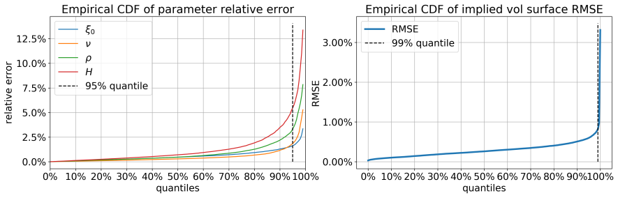
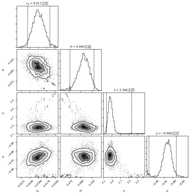
The central claim is that a neural network trained off-line to reproduce a model's implied volatility map can stand in for the model's slow numerical pricing engine during calibration, without sacrificing the interpretability or risk-management structure of the underlying model. The demonstration is on the rough Bergomi model, a non-Markovian stochastic volatility model whose volatility is driven by fractional Brownian motion with Hurst parameter below 1/2, making each Monte Carlo price expensive. With a three-hidden-layer, 30-neuron network whose output is an 8-by-11 grid of implied volatilities, calibrating the full rough Bergomi surface is reported to take less than 40 milliseconds; across the test set, the 99% quantile of the root-mean-square surface error is below 1% and the maximum surface RMSE is below 4%. The paper also shows that the same network enables Bayesian calibration against both synthetic and SPX market implied volatility surfaces, producing posterior distributions whose peaks lie close to the true or previously reported parameter values.
Load-bearing premise
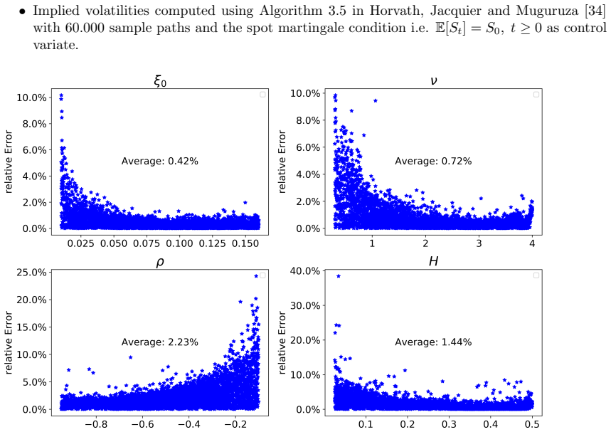
The pipeline inherits the accuracy of the Monte Carlo scheme that produced the training labels: if that scheme is biased for rough Bergomi prices, especially at short maturities and extreme strikes where the paper reports relative errors up to 25%, the neural network learns that bias and successful synthetic calibration only shows self-consistency with the Monte Carlo generator.
Editorial extensions
If this is right
- Rough Bergomi, which is notoriously slow to calibrate by Monte Carlo, can be calibrated in under 40 milliseconds on a standard CPU, making on-the-fly calibration practically feasible.
- Because the network is trained on synthetic model data rather than market data, it does not need to be retrained when market regimes change; only the second optimization step is market-dependent.
- The same two-step architecture transfers to other stochastic volatility models, with simpler networks sufficient for models such as SABR and Heston and deeper networks needed for rough models.
- The nearly instantaneous pricing map makes Bayesian calibration practical, allowing posterior distributions over model parameters to be sampled by MCMC at very low computational cost.
- Risk management and model interpretation remain intact because the neural network only replaces the numerical pricing engine; its outputs are still model implied volatilities with standard Jacobians.
Reading between the lines
- We infer that the same two-step recipe extends naturally to a non-constant forward variance curve, whose piecewise-constant parameters would simply enlarge the network's input dimension; the paper lists this as future work.
- We infer that focusing training samples or loss weights on the error zones the paper reports, namely short maturities and deep out-of-the-money or in-the-money strikes, would likely reduce the maximum 25% relative errors, which occur precisely where the Monte Carlo labels are least reliable.
- We infer that the reported speedup changes calibration from a batch end-of-day computation into an intraday or streaming task, since a 40-millisecond full-surface fit can be repeated thousands of times within a trading session.
Signed reviews
Editorial analysis
A structured set of objections, weighed in public.
Referee Report
Summary. The paper proposes a two-step deep calibration pipeline for stochastic volatility models, with the rough Bergomi model as the main test case. In the first step, a neural network is trained offline to approximate the model's implied-volatility map, either pointwise in option parameters or in a grid-based 'implicit' mode. In the second step, the fast surrogate is used inside a standard Levenberg-Marquardt calibration or a Bayesian MCMC procedure. The authors report a full-surface neural-network evaluation time of about 14 microseconds (21,000–35,000 times faster than their Monte Carlo benchmark), calibration times below 40 milliseconds for the rough Bergomi model, small RMSE on synthetic test surfaces, and posterior concentration near true parameters in a Bayesian experiment. They also compare this two-step approach with a one-step inverse-map neural network and find that the inverse map generalizes poorly to out-of-sample data.
Significance. If the accuracy claims hold, this is a practically valuable contribution: it separates the neural component from the calibration step, allows automatic differentiation of the pricing map, uses a small CPU-friendly network (5,668 parameters), and makes Bayesian calibration feasible for rough volatility models. The comparison of pointwise vs. grid-based training and the out-of-sample inverse-map experiment are useful for practitioners. The main caveat is that the numerical validation is currently self-referential: both the training labels and the synthetic calibration targets are produced by the same Monte Carlo scheme, so the reported accuracy is conditional on that scheme being unbiased. The paper does not provide an independent pricing benchmark or Monte Carlo error quantification, which is the key weakness for the central 'sufficient accuracy for practical use' claim.
major comments (3)
- [§5.1–§5.3, Figs. 2, 5, 6] The synthetic validation is circular with respect to the Monte Carlo generator. Section 5.1 states that training labels are computed with Algorithm 3.5 of Horvath, Jacquier and Muguruza [34] using 60,000 paths, and Sections 5.2 and 5.3 generate the test IV surfaces 'using Monte Carlo simulation as in Section 5.2 above'. Thus Figures 4–6 and the reported 99% RMSE quantile below 1% measure the network's ability to invert this particular Monte Carlo scheme, not its accuracy against the true rough Bergomi pricing map. The manuscript acknowledges in Section 5.1 that maximum network-vs-MC relative errors reach 25% and that these are 'consistent with the errors of the Monte Carlo training set', which explicitly makes the MC label error the floor of the reported accuracy. Since no MC bias quantification or independent pricing benchmark is provided, the central practical-accuracy claim is not yet established. Please add MC confidence intervals or a comparison with a second pricing method (e.g., the hybrid scheme of Bennedsen–Lunde–Pakkanen or asymptotic expansions) at the short-maturity and extreme-strike locations where the largest errors occur.
- [§5.3, Fig. 7] The SPX market-data Bayesian experiment is the only test not generated by the same Monte Carlo scheme, but it is reported only as posterior histograms. No comparison is made with parameters obtained by direct Monte Carlo calibration, no surface fit RMSE is reported, and no quantitative measure of how well the posterior matches the market data is given. As a result, Figure 7 cannot independently support the accuracy claim; it only shows that the procedure produces parameter regions that look plausible. Please report the calibrated surface error and, if possible, compare the posterior mode/median with a benchmark calibration obtained by a standard numerical pricer.
- [§4.2.1, Figs. 6–7] The Bayesian credible intervals depend on the assumed error scale, but the paper does not report the prior distributions or the specific values of σ_i used in the likelihood beyond 'a fractional of the spread'. The posterior widths in Figures 6–7 are therefore hard to interpret. Please state the priors and the exact heteroskedastic error specification, and include a sensitivity check to the choice of σ_i.
minor comments (6)
- [§5.1] The text refers to 'Algorithm 3.5 in Horvath, Jacquier and Muguruza [34]' as if it were available in this paper; since Algorithm 3.5 is not defined here, the reference should be made explicit in the sentence.
- [§2, Eq. (2) and Algorithm 1] The normal equations use J(µ_k) where the iteration variable µ_k is undefined; the Jacobian should presumably be evaluated at θ_k, so the notation should be J(θ_k).
- [§3.2.1, Eq. (5)] The network is written as F(w;θ,T,k) in equation (5) but as F(w;θ,ζ) in the surrounding text; unify the notation for readability.
- [§3.2.1] The sentence 'to obtain even higher accuracy, one could also choose a coarser grid, which would require longer learning time' appears to state the opposite of what is intended; likely 'finer grid' was meant.
- [Abstract, §5.2, references] The manuscript contains several typos: 'on the y' should be 'on the fly', 'Tabe 1' should be 'Table 1', 'accuarcy' should be 'accuracy', and in the reference list [15] 'neworks' should be 'networks' and [41] should be 'Kingma and Ba' rather than 'Kingman and Ba'.
- [§5.2] The statement that calibration times 'usually under 10 milliseconds' for Markovian stochastic volatility models is not supported by any experiment in this paper; please either provide data or soften the claim.
Circularity Check
No significant circularity: the two-step calibration benchmark is a held-out surrogate test, and the SPX market calibration is independent.
full rationale
The paper's derivation chain is not circular. The neural network is trained on Monte Carlo labels produced by Algorithm 3.5 of Horvath, Jacquier and Muguruza [34], and the synthetic calibration and Bayesian experiments generate test data with the same scheme, but the network is not fitted to those test parameter points: the test set is held out and the synthetic experiments measure whether the learned map, at new parameters, inverts the generator. This is a standard supervised-learning benchmark, not a fitted input renamed as a prediction. The true-model accuracy of the labels is an external numerical-analysis question, and the paper explicitly acknowledges that the maximum network-vs-MC errors are "consistent with the errors of the Monte Carlo training set," i.e., it does not claim to validate the MC scheme itself. Moreover, the SPX market-data calibration in Section 5.2/5.3 and the comparative inverse-map experiment in Appendix A provide independent, non-self-referential evidence: the market surface is not generated by the same Monte Carlo code, and the inverse-map generalization failure is measured against brute-force Monte Carlo. The self-citations to predecessor papers [7] and [35] and to the paper's own MC algorithm [34] are normal methodological references; no uniqueness theorem is imported, no ansatz is smuggled in via self-citation, and no central claim reduces by construction to its inputs. The reader's concern about MC bias is a legitimate correctness/validation risk, but it is not circularity under the criteria of this pass.
Assumptions & free parameters
free parameters (4)
- Neural network weights (5,668 parameters) =
Trained on 34,000 Monte Carlo surfaces
- Training parameter ranges =
xi0 in [0.01,0.16], nu in [0.5,4.0], rho in [-0.95,-0.1], H in [0.025,0.5]
- MC training path count and grid =
60,000 paths; 11 strikes by 8 maturities
- Network architecture and optimization hyperparameters =
3 hidden layers of 30 nodes, ELU activation, Adam optimizer
assumptions (6)
- domain assumption Algorithm 3.5 in [34] provides sufficiently accurate approximate prices for the rough Bergomi model.
- domain assumption The implied volatility surface is smooth enough for spline interpolation between grid points.
- domain assumption The chosen uniform parameter ranges cover realistic market scenarios.
- standard math Multilayer neural networks can approximate the pricing map.
- domain assumption The Bayesian regression error is normally distributed.
- domain assumption The market implied volatility surface is generated by the rough Bergomi model up to liquidity noise.
Cite this review
Pith. "Pith review of On deep calibration of (rough) stochastic volatility models." pith.science (2026). https://pith.science/paper/CHON4WMJ
@misc{pith2026190808806,
  author       = {Pith},
  title        = {Pith review of: On deep calibration of (rough) stochastic volatility models},
  year         = {2026},
  howpublished = {\url{https://pith.science/paper/CHON4WMJ}},
  note         = {Machine review of arXiv:1908.08806}
}
read the original abstract
Techniques from deep learning play a more and more important role for the important task of calibration of financial models. The pioneering paper by Hernandez [Risk, 2017] was a catalyst for resurfacing interest in research in this area. In this paper we advocate an alternative (two-step) approach using deep learning techniques solely to learn the pricing map -- from model parameters to prices or implied volatilities -- rather than directly the calibrated model parameters as a function of observed market data. Having a fast and accurate neural-network-based approximating pricing map (first step), we can then (second step) use traditional model calibration algorithms. In this work we showcase a direct comparison of different potential approaches to the learning stage and present algorithms that provide a suffcient accuracy for practical use. We provide a first neural network-based calibration method for rough volatility models for which calibration can be done on the y. We demonstrate the method via a hands-on calibration engine on the rough Bergomi model, for which classical calibration techniques are diffcult to apply due to the high cost of all known numerical pricing methods. Furthermore, we display and compare different types of sampling and training methods and elaborate on their advantages under different objectives. As a further application we use the fast pricing method for a Bayesian analysis of the calibrated model.
Figures


Figures from the paper (6 more)



Forward citations
Cited by 2 Pith papers
-
Signature-based identification of volatility models from path geometry
Truncated path signatures combined with XGBoost classify stochastic volatility model classes from simulated paths with high accuracy, including under random parameter variation and closely spaced Hurst parameters.
-
Deep learning interpretability for rough volatility
A neural network trained to invert rough Heston parameters from implied volatility surfaces relies most on short-maturity deep in-the-money prices, a pattern absent in the standard Heston model.
Reference graph
Works this paper leans on
-
[34]
Functional central limit theorems for rough volatility
B. Horvath, A. Jacquier and A. Muguruza. Functional central limit theorems for rough volatil- ity. arXiv:1711.03078, 2017
work page Pith review arXiv 2017
-
[53]
H. Stone. Calibrating rough volatility models: a convolutional neural network approach. Preprint, arXiv:1812.05315, 2018. 32
work page Pith review arXiv 2018
- [1]
-
[2]
A. Antonov, M. Konikov, M. Spector. Modern SABR Analytics: Formulas and Insights for Quants, Former Physicists and Mathematicians. SpringerBriefs in Quantitative Finance, 2019
work page 2019
-
[3]
M. Avellaneda, A. Carelli, F. Stella. Following the Bayes path to option pricing. Journal of Computational Intelligence in Finance , 84, 1999
work page 1999
-
[4]
A regularity structure for rough volatility
C. Bayer, P. Friz, P. Gassiat, J. Martin and B. Stemper. A regularity structure for rough volatility. arXiv:1710.07481, 2017
work page Pith review arXiv 2017
- [5]
-
[6]
Short-time near-the-money skew in rough fractional volatility models
C. Bayer, P. Friz, A. Gulisashvili, B. Horvath and B. Stemper. Short-time near the money skew in rough fractional stochastic volatility models. arXiv:1703.05132, 2017
work page Pith review arXiv 2017
Show all 53 references
-
[7]
Bayer and B
C. Bayer and B. Stemper. Deep calibration of rough stochastic volatility models. Preprint, arXiv:1810.03399
-
[8]
Bennedsen, A
M. Bennedsen, A. Lunde and M.S. Pakkanen. Hybrid scheme for Brownian semistationary processes. Finance and Stochastics, 21(4): 931-965, 2017
2017
-
[9]
L. Bergomi. Stochastic Volatility Modeling. Chapman & Hall/CRC financial mathematical series. Chapman & Hall/CRC , 2015
2015
-
[10]
B. Chen, C. W. Oosterlee and H. Van Der Weide. Efficient unbiased simulation scheme for the SABR stochastic volatility model, 2011
2011
-
[11]
R. Cont. Model Calibration. Encyclopedia of Quantitative Finance , 5, 2010. DOI:10.1002/9780470061602.eqf08002
2010 doi
-
[12]
Culkin and S
R. Culkin and S. R. Das Machine Learning in Finance: The Case of Deep Learning for Option Pricing. Journal of Investment Management , github:BlackScholesNN 2017. 29
2017
-
[13]
De Spiegeleer, D
J. De Spiegeleer, D. Madan, S. Reyners and W. Schoutens. Machine learning for quantitative finance: Fast derivative pricing, hedging and fitting. SSRN:3191050, 2018
2018
-
[14]
Dimitroff, D
G. Dimitroff, D. R¨ oder and C. P. Fries. Volatility model calibration with convolutional neural networks. Preprint, SSRN:3252432, 2018
2018
-
[15]
Eldan and O
R. Eldan and O. Shamir. The power of depth for feedforward neural neworks.JMLR: Workshop and Conference Proceedings Vol 49:1-34 , 2016
2016
-
[16]
El Euch and M
O. El Euch and M. Rosenbaum. Perfect hedging in rough Heston models, to appear in The Annals of Applied Probability, 2018
2018
-
[17]
Forde, H
M. Forde, H. Zhang. Asymptotics for Rough Stochastic Volatility
-
[18]
Friedman, R
J. Friedman, R. Tibshiran and T. Hastie. The Elements of Statistical Learning. Springer New York Inc, 2001
2001
-
[19]
Ferguson and A
R. Ferguson and A. D. Green. Deeply learning derivatives. Preprint arXiv:1809.02233, 2018
2018 arXiv
-
[20]
Foreman-Mackey, D
D. Foreman-Mackey, D. W. Hogg, D. Lang, J. Goodman. emcee: the MCMC hammer, Publi- cations of the Astronomical Society of the Pacific , 125(925), 306, 2013
2013
-
[21]
Foreman-Mackey, corner.py: Scatterplot matrices in Python, The Journal of Open Source Software 24, http://dx.doi.org/10.5281/zenodo.45906, 2016
D. Foreman-Mackey, corner.py: Scatterplot matrices in Python, The Journal of Open Source Software 24, http://dx.doi.org/10.5281/zenodo.45906, 2016
2016 doi
-
[22]
Fukasawa
M. Fukasawa. Asymptotic analysis for stochastic volatility: martingale expansion. Finance and Stochastics, 15: 635-654, 2011
2011
-
[23]
Gatheral
J. Gatheral. The volatility surface: a practitioner’s guide, Wiley, 2011
2011
-
[24]
Gatheral, T
J. Gatheral, T. Jaisson and M. Rosenbaum. Volatility is rough. Quantitative Finance, 18(6): 933-949, 2018
2018
-
[25]
K. Glau, D. Kressner, and F. Statti. Low-rank tensor approximation for Chebyshev interpola- tion in parametric option pricing. arXiv:1902.04367, 2019
1902 arXiv
-
[26]
A. Green. XVA: Credit, Funding and Capital Valuation Adjustments. Wiley, 2015
2015
-
[27]
Hagan, D
P. Hagan, D. Kumar, A. Lesniewski, and D. Woodward. Managing smile risk. Wilmott Maga- zine, September issue: 84-108 , 2002
2002
-
[28]
J. Han, A. Jentzen, E. Weinan. Overcoming the curse of dimensionality: Solving high- dimensional partial differential equations using deep learning. PNAS.115(34) 8505-8510, Au- gust 2018
2018
-
[29]
S.L. Heston. A closed-form solution for options with stochastic volatility with applications to bond and currency options, The Review of Financial Studies 6(2):327–343, 1993
1993
-
[30]
Hernandez
A. Hernandez. Model calibration with neural networks. Risk, 2017
2017
-
[31]
Hornik, M
K. Hornik, M. Stinchcombe, and H. White. Multilayer feedforward networks are universal approximators. Neural Networks, 2(5):359-366, 1989
1989
-
[32]
K. Hornik. M. Stinchcombe and H. White. Universal approximation of an unknown mapping and its derivatives using multilayer feedforward networks. Neural Networks. Vol. 3:11, 1990. 30
1990
-
[33]
Henry-Labord` ere
P. Henry-Labord` ere. Deep primal-dual algorithm for BSDEs: applications of machine learning to CVA and IM. SSRN:3071506
-
[35]
Horvath, A
B. Horvath, A. Muguruza and T. Mehdi. Deep learning volatility. Available at SSRN 3322085, 2019
2019
-
[36]
Horvath, O
B. Horvath, O. Reichmann. Dirichlet Forms and Finite Element Methods for the SABR Model. SIAM Journal on Financial Mathematics , p. 716-754 (2), May 2018
2018
-
[37]
Hull and A
J. Hull and A. White. Pricing interest rate derivatives securities. The Review of Financial Studies)(3): 573-592, 1990
1990
-
[38]
J. M. Hutchinson, A. W. Lo and T. Poggio. A Nonparametric Approach to Pricing and Hedging Derivative Securities Via Learning Networks. The Journal of Finance , 49(3) 851-889. Papers and Proceedings Fifty-Fourth Annual Meeting of the American Finance Association, Boston, Massac...
1994
-
[39]
A. Itkin. To sigmoid-based functional description of the volatility smile. Preprint, arXiv:1407.0256, 2014
2014 arXiv
-
[40]
Ioffe and C
S. Ioffe and C. Szegedy. Batch normalisation: Accelerating deep network training by reducing internal covariate shift. Preprint, arXiv:1502.03167, 2015
2015 arXiv
-
[41]
Kingman and J
D.P. Kingman and J. Ba, Adam: A Method for Stochastic Optimization. Conference paper, 3rd International Conference for Learning Representations, 2015
2015
-
[42]
Leitao Rodriguez, L.A
A. Leitao Rodriguez, L.A. Grzelak and C.W. Oosterlee. On an efficient multiple time step Monte Carlo simulation of the SABR model.Quantitative Finance, 17(10), pp.1549-1565, 2017
2017
-
[43]
Levenberg
K. Levenberg. A Method for the Solution of Certain Non-Linear Problems in Least Squares. Quarterly of Applied Mathematics . 2: pp. 164-168, 1944
1944
-
[44]
Marquardt
D. Marquardt. An Algorithm for Least-Squares Estimation of Nonlinear Parameters. SIAM Journal on Applied Mathematics . 11 (2): pp. 431-441,1963.‘
1963
-
[45]
S. Liu, A. Borovykh, L. A. Grzelak, C. W. Oosterlee. A neural network-based framework for financial model calibration. Preprint, arXiv:1904.10523, 2019
1904 arXiv
-
[46]
W. A. McGhee. An artificial neural network representation of the SABR stochastic volatility model. Preprint, SSRN:3288882, 2018
2018
-
[47]
McCrickerd, M
R. McCrickerd, M. Pakkanen, Turbocharging Monte Carlo pricing for the rough Bergomi model, Quantitative Finance 18(11):1877-1886, 2018
2018
-
[48]
Leitao Rodriguez, A
A. Leitao Rodriguez, A. Grzelak Lech, Cornelis W. Oosterlee. On a one time-step Monte Carlo simulation approach of the SABR model : Application to European options. Applied Mathematics and Computation , 293 p. 461-479, 2017,
2017
-
[49]
Sabate Vidales, D
M. Sabate Vidales, D. Siska, L. Szpruch Unbiased deep solvers for parametric PDEs arXiv:1810.05094, 2018. 31
2018 arXiv
-
[50]
Sirignano and K
J. Sirignano and K. Spiliopoulos. DGM: A deep learning algorithm for solving partial differ- ential equations. Journal of Computational Physics 375(15) 1339-1364, December 2018
2018
-
[51]
Setayeshgar, and H
L. Setayeshgar, and H. Wang. Large deviations for a feed-forward network,Advances in Applied Probability, 43: 2, pp. 545-571, 2011
2011
-
[52]
Shaham, A
U. Shaham, A. Cloninger, and R. R. Coifman. Provable approximation properties for deep neural networks. Appl. Comput. Harmon. Anal. , 44(3): 537-557, 2018
2018
Reviewed August 14, 2026 · model on record in the stance chip above.
Discussion (0). Continue with ORCID to comment.