REVIEW 2 major objections 4 minor 3 cited by
Ensemble Average of Three-Dimensional Minkowski Tensors of a Gaussian Random Field in Redshift Space
T0 review · 2 major / 4 minor · reviewed 2026-08-14 · deepseek-v4-flash
Pith's one-line read Closed-form ensemble averages for Minkowski tensors in redshift space yield ratio observables that isolate the growth-rate parameter β.
desk verdict First analytic ensemble prediction for 3D Minkowski tensors in redshift space, numerically validated at the 1% level; the new β-only ratios are a real step forward, but the unstated redefinition of the threshold ν needs a one-sentence fix. read the letter →
The pith
A machine-rendered reading of the paper's core claim, the machinery that carries it, and where it could break.
The reading
What carries the argument
The machinery is the boundary-integral representation of the Minkowski tensors: $W^{0,2}_1$ is an integral over iso-density surfaces of the symmetric product of the unit normal, and $W^{0,2}_2$ weights the same integrand by the mean curvature; both are normalized by the survey volume. For a Gaussian field these become integrals over a multivariate Gaussian distribution of the field value, its first derivatives, and its second derivatives, with the excursion-set threshold enforced by a delta function. Redshift-space distortion enters through the Kaiser factor $(1+\beta\mu^2)^2$ in the power spectrum, which changes the field cumulants $\sigma_0$, $\sigma_{1\perp}$, $\sigma_{1\parallel}$, $\sigma_{2\perp}$, $\sigma_{2\parallel}$, and $\sigma_{2\times}$; the only combination that survives in the diagonal ratios is $\lambda^2 = \sigma^2_{1\parallel}/\sigma^2_{1\perp} = (35+42\beta+15\beta^2)/(35+14\beta+3\beta^2)$. The argument proceeds by decorrelating the second-derivative variables through linear transformations and showing that all terms involving them integrate to zero, leaving the closed forms (46)-(49).
What would settle it
Measure the diagonal ratios $\Theta_{1|I}$ and $\Theta_{2|I}$ from a large N-body simulation with a known growth rate and bias, on scales where the field should be Gaussian; if the measured ratios deviate from equations (51)-(52) by more than the simulation's statistical error, the central claim is wrong.
Extended reading notes
Core claim
The authors claim that for a Gaussian random field whose power spectrum is modified by the linear Kaiser factor, the ensemble averages of $W^{0,2}_1$ and $W^{0,2}_2$ are diagonal matrices with explicit closed forms (46)-(49). The anisotropy introduced by redshift-space distortion makes the entry along the line of sight (index 3) differ from the two perpendicular entries (index $I=1,2$). Because the prefactors involving the real-space cumulants $\sigma_0$, $\sigma_1$, and $\sigma_2$ cancel, the ratios $a_{1|I}/a_{1|3}$ and $a_{2|I}/a_{2|3}$ depend only on the single parameter $\lambda^2=\sigma^2_{1\parallel}/\sigma^2_{1\perp}$, which is itself a rational function of $\beta=f/b$. Thus the diagonal ratios isolate $\beta$ from all other cosmological parameters. The paper further argues that these ratios should be measured from the matrix elements directly rather than from the eigenvalues of the tensors, because eigenvalue ratios acquire a noise-induced bias in the isotropic limit that is not under analytic control.
Load-bearing premise
The derivation assumes that the redshift-space density field is exactly Gaussian with the linear Kaiser power spectrum in the distant-observer limit; if non-Gaussian velocity effects or wide-angle geometry are significant, the analytic formulas do not apply.
Editorial extensions
If this is right
- Galaxy surveys can use $\Theta_{1|I}$ and $\Theta_{2|I}$ as cosmological observables that isolate $\beta=f/b$ without needing to know the clustering amplitude or bias separately.
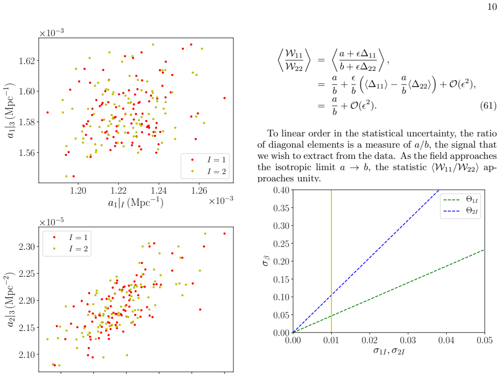
- $W^{0,2}_1$ is the more powerful of the two statistics: a one percent measurement of its diagonal ratio yields roughly a four percent constraint on $\beta$, while the same accuracy in $W^{0,2}_2$ yields about a ten percent constraint.
- Matrix elements, not eigenvalues, should be used for parameter estimation when the anisotropy direction is known; eigenvalue ratios can masquerade as anisotropy in an isotropic field purely from statistical noise.
- The analytic predictions hold only for linear distortions in the distant-observer limit; extending them to non-Gaussian or wide-angle regimes requires corrections beyond this work.
Reading between the lines
- If the ratio method is as clean as claimed, it could be applied to other anisotropic signals with a known direction, such as intrinsic alignments or survey window functions, by measuring diagonal ratios of Minkowski tensors in a coordinate system aligned with that direction.
- The eigenvalue caveat suggests a general test for any shape statistic defined through eigen-decompositions: check whether its expectation value in an isotropic field with finite noise differs from the isotropic signal, since a nonzero offset would mimic anisotropy.
- The same derivation chain could produce analogous ratios for higher-rank Minkowski tensors or for translation-covariant tensors, potentially giving additional independent constraints on $\beta$ from the same survey data.
- Comparing the Gaussian prediction with ratios measured from simulations that include gravitational non-Gaussianity would map the scale and smoothing range where the $\beta$-only dependence survives, which is a testable extension.
Editorial analysis
A structured set of objections, weighed in public.
Referee Report
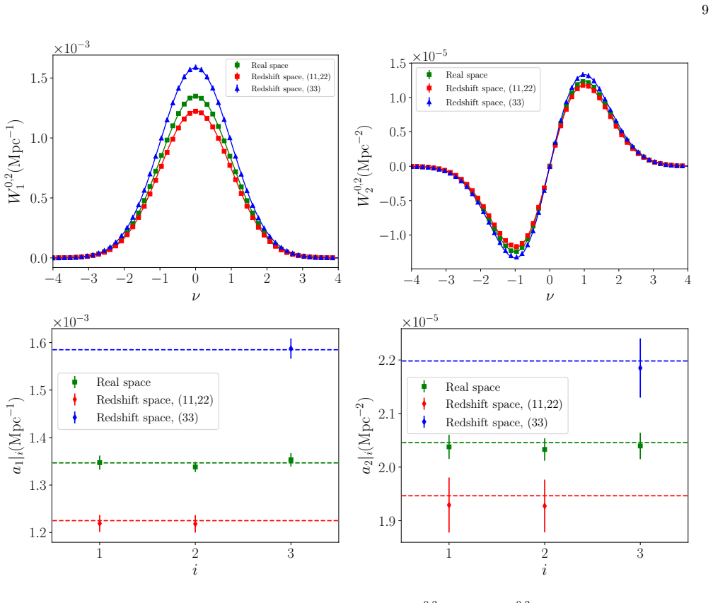
Summary. The paper derives ensemble-averaged values for the translation-invariant rank-2 Minkowski tensors W_1^{0,2} and W_2^{0,2} for a three-dimensional Gaussian random field subject to linear Kaiser redshift-space distortion. Section II reviews the isotropic real-space calculation; Section III generalizes it to a field with line-of-sight-dependent cumulants, obtaining diagonal but unequal expectation values (Eqs. (28)-(29), (39)-(40)) and the amplitude coefficients (46)-(49). The ratios Theta_{1|I} and Theta_{2|I} of perpendicular and parallel amplitudes are shown to depend only on beta=f/b. Section IV validates the analytic predictions against 100 numerical Gaussian realizations with agreement better than about 1%, and Section V argues for using the matrix elements rather than eigenvalue ratios for cosmological parameter estimation.
Significance. The paper provides closed-form, parameter-free (given beta) predictions for Minkowski-tensor amplitudes in redshift space, and the cancellation of all cosmological parameters except beta in the ratios is a strong and useful feature. The numerical confirmation of the analytic results at sub-percent level is a genuine external check and strengthens confidence in the derivation. The clear statement of the linear-Kaiser/Gaussian scope is appropriate, and the comparison of matrix-element versus eigenvalue statistics is a useful practical contribution. If the threshold normalization ambiguity is resolved, these results constitute a practical tool for extracting redshift-space distortion constraints from morphological statistics of galaxy surveys.
major comments (2)
- [Section III, Eq. (27)] The threshold variable nu is defined in Section II as nu = delta_c/sigma_0, but in Section III the field is renormalized as x = delta/sigma with sigma^2 = A_0 sigma_0^2, and Eq. (27) writes delta_D(x-nu) without redefining nu. Consistency requires nu = delta_c/sigma, using the redshift-space variance, not delta_c/sigma_0. As written, the predicted curves W_i(nu) in Eqs. (28)-(29) and (39)-(40) are expressed in ambiguous threshold units; a reader adopting the Section II definition would obtain incorrect absolute predictions. The ratios (51)-(52) are not affected because the sigma-dependent prefactors cancel, but the central formulas (46)-(49) and their derivation are only unambiguous once the threshold redefinition is stated. Please add an explicit one-sentence redefinition of nu after Eq. (23) and use it consistently throughout.
- [Section IV, numerical analysis] The numerical validation does not state which variance is used to normalize the threshold when comparing the anisotropic-field measurements with the analytic curves. The reported agreement below 1% suggests that the redshift-space variance sigma_s was used, but this must be stated explicitly for the test to be reproducible. If instead the real-space sigma_0 were used to set nu, the amplitudes extracted via Eqs. (54)-(55) would be rescaled by (sigma_s/sigma_0)^n relative to Eqs. (46)-(49), and the comparison with the analytic predictions would not be meaningful. Please specify the variance normalization used for the threshold in both the isotropic and anisotropic fields.
minor comments (4)
- [Section I] There is a typo in the introduction: 'Minkowki' should be 'Minkowski'.
- [Section III, after Eq. (23)] It would help the reader to denote the redshift-space variance explicitly, for example sigma_s^2 = A_0 sigma_0^2, so that it is clearly distinguished from the real-space sigma_0 throughout.
- [Section IV, Figure 1] Please specify the orientation of the box and the line-of-sight axis used in the numerical simulations, since the analytic results are only valid when the line of sight is aligned with one coordinate axis.
- [Section IV, Eqs. (57)-(58)] The term 'optimistically' is appropriate for the single-parameter Fisher-type bound, but it would be useful to state explicitly that this forecast assumes no other nuisance parameters and ignores any residual correlation between the amplitude estimates.
Circularity Check
No significant circularity: the redshift-space Minkowski tensor predictions are derived from the stated Gaussian/Kaiser model and tested against independent simulations.
full rationale
The central result (Eqs. 46-49) is obtained by direct analytic integration of the Gaussian probability functional with the linearly redshift-space-distorted cumulants (Eqs. 23-25). The A factors are fixed by the Kaiser-model power spectrum P_s(k) = (1+β μ^2)^2 P(k), not fitted to the Minkowski-tensor outputs; no parameter is calibrated from the quantities being predicted. The ratios Θ1|I and Θ2|I are formed after deriving the amplitudes, and the cancellation of the σ prefactors follows algebraically, so the β-only dependence is a consequence rather than an input. The numerical simulations in Sec. IV serve as an independent test of the formulas, and the self-citations (e.g., ref. [50] for numerical reconstruction and refs. [49,50] for the isotropic expectation values) are not load-bearing: the isotropic case is re-derived in Sec. II A from the Gaussian probability distribution, and the reconstruction method is used only to validate, not to define, the prediction. There is therefore no step in which a prediction is equivalent by construction to a fitted input or to an unverified self-citation. The ν-normalization ambiguity noted by a skeptical reader (whether ν is δc/σ0 or δc/σ after the redefinition x = δ/σ in Sec. III) is a potential correctness/application issue, but it is not circularity: it does not make Eqs. (46-49) identical to any input assumption.
Assumptions & free parameters
assumptions (5)
- domain assumption The matter density field is a Gaussian random field with a given power spectrum P(k).
- domain assumption Linear Kaiser redshift-space distortion in the plane-parallel limit: δ_s(k) = (1+β μ²) δ_r(k), with β = f/b.
- domain assumption The Minkowski tensor statistics of the redshift-space field can be computed from the field and its derivatives in redshift-space coordinates using the standard Gaussian random field formalism.
- standard math The coarea formula / integral transformation (eq. 6) relating surface integrals to volume integrals with a delta function.
- domain assumption Statistical homogeneity and ergodicity of the field, so the volume average equals the ensemble average.
Cite this review
Pith. "Pith review of Ensemble Average of Three-Dimensional Minkowski Tensors of a Gaussian Random Field in Redshift Space." pith.science (2026). https://pith.science/paper/CYDVW6M6
@misc{pith2026190802440,
  author       = {Pith},
  title        = {Pith review of: Ensemble Average of Three-Dimensional Minkowski Tensors of a Gaussian Random Field in Redshift Space},
  year         = {2026},
  howpublished = {\url{https://pith.science/paper/CYDVW6M6}},
  note         = {Machine review of arXiv:1908.02440}
}
abstract
We present the ensemble expectation values for the translation invariant, rank-2 Minkowski tensors in three-dimensions, for a linearly redshift space distorted Gaussian random field. The Minkowski tensors $W^{0,2}_{1}$, $W^{0,2}_{2}$ are sensitive to global anisotropic signals present within a field, and by extracting these statistics from the low redshift matter density one can place constraints on the redshift space distortion parameter $\beta = f/b$. We begin by reviewing the calculation of the ensemble expectation values $\langle W^{0,2}_{1} \rangle$, $\langle W^{0,2}_{2} \rangle $ for isotropic, Gaussian random fields, then consider how these results are modified by the presence of a linearly anisotropic signal. Under the assumption that all fields remain Gaussian, we calculate the anisotropic correction due to redshift space distortion in a coordinate system aligned with the line of sight, finding inequality between the diagonal elements of $\langle W^{0,2}_{1} \rangle $, $\langle W^{0,2}_{2} \rangle $. The ratio of diagonal elements of these matrices provides a set of statistics that are sensitive only to the redshift space distortion parameter $\beta$. We estimate the Fisher information that can be extracted from the Minkowski tensors, and find $W^{0,2}_{1}$ is more sensitive to $\beta$ than $W^{0,2}_{2}$, and a measurement of $W^{0,2}_{1}$ accurate to $\sim 1\%$ can yield a $\sim 4\%$ constraint on $\beta$. Finally, we discuss the difference between using the matrix elements of the Minkowski tensors directly against measuring the eigenvalues. For the purposes of cosmological parameter estimation we advocate the use of the matrix elements, to avoid spurious anisotropic signals that can be generated by the eigenvalue decomposition.
Figures
Forward citations
Cited by 3 Pith papers
-
Testing Statistical Isotropy on the Sphere with Minkowski Tensors
Connected-patch orientation correlations ξ±(θ,ν) give a coordinate-independent test of statistical isotropy on the sphere and separate global from local alignment in sheared random fields, while dipole modulation leav...
-
Cosmological constraints from the Minkowski functionals of the BOSS CMASS galaxy sample
A simulation-based emulator of Minkowski functionals applied to BOSS CMASS galaxies yields cosmological constraints from both Gaussian and non-Gaussian information, tighter than the 2PCF alone.
-
Probing massive neutrinos and modified gravity with redshift-space morphologies and anisotropies of large-scale structure
In a dark-matter-only simulation forecast, combining power spectrum multipoles with Minkowski functionals and tensors tightens constraints on neutrino mass and f(R) gravity parameters by factors of 1.5 to 3.4.
Reference graph
Works this paper leans on
-
[1]
H. Hadwiger, Vorlesungen ber Inhalt, Oberflche und Isoperimetriee (Springer, Grundlehren der mathematis- chen Wissenschaften, 1957)
work page 1957
-
[2]
Matheron, Random sets and integral geometry (Wiley New York, 1974)
G. Matheron, Random sets and integral geometry (Wiley New York, 1974)
work page 1974
-
[3]
= σ1 9 √ 3πσ0 e−ν2/2. (14) The isotropy of the field has manifested as ⟨W 0,2 1 ⟩ being proportional to the identity matrix – all diagonal ele- ments are equal. The integrand of⟨W 0,2 2 ⟩ contains all ten variables. To proceed, we de-correlate xii andx using the linear trans- formation 4 yii = xii +γx√ 1−γ2. (15) The mean curvatureG2 is then given in terms...
-
[4]
˜M|II ˜X4 [ (x2 1 +x2 2)(1 +λ2) + 2λ2x2 3 ] , (37) ⟨W 0,2 2 |33⟩ = σ2 1⊥νe−ν2/2 72π3σ2 ∫ ∞ −∞ dx1 ∫ ∞ −∞ dx2 ∫ ∞ −∞ dx3e− 1 2(x2 1+x2 2+x2
-
[5]
˜M|33 ˜X4 [ (x2 1 +x2 2)(1 +λ2) + 2λ2x2 3 ] . (38) The integrals admit analytic solutions ⟨W 0,2 2 |II⟩ = σ2 1⊥ 72π √ 2πσ2 [ (λ2− 2)(λ2− 1)1/2 +λ4 tan−1√ λ2− 1 ] (λ2− 1)3/2 νe−ν2/2, (39) ⟨W 0,2 2 |33⟩ = σ2 1⊥ 36π √ 2πσ2 λ2[ (λ2− 1)1/2 + (λ2− 2) tan−1√ λ2− 1 ] (λ2− 1)3/2 νe−ν2/2, (40) ⟨W 0,2 2 |IJ⟩ = ⟨W 0,2 2 |I3⟩ = 0. (41) In the isotropic limit, β → 0, λ...
work page 2018
-
[6]
D. Hug, R. Schneider, and R. Schuster, St. Petersburg Math. J. 19, 137 (2008)
work page 2008
- [7]
-
[8]
Alesker, Geometriae Dedicata 74, 241 (1999)
S. Alesker, Geometriae Dedicata 74, 241 (1999)
work page 1999
Show all 67 references
-
[9]
Beisbart, R
C. Beisbart, R. Dahlke, K. Mecke, and H. Wagner, in Morphology of Condensed Matter (2002), vol. 600 of Lec- ture Notes in Physics, Berlin Springer Verlag , pp. 238– 260
2002
-
[10]
L. A. Santalo, Integral geometry and geometric probabil- ity (Addison-Wesley Pub. Co., Advanced Book Program Reading, Mass, 1976)
1976
-
[11]
G. E. Schroder-Turk, W. Mickel, S. C. Kapfer, F. M. Schaller, B. Breidenbach, D. Hug, and K. Mecke, New Journal of Physics 15, 083028 (2013)
2013
-
[12]
Schroder-Turk, S
G. Schroder-Turk, S. Kapfer, B. Breidenback, C. Beis- bart, and K. Mecke, Journal of Microscopy 238, 57 (2010), ISSN 1365-2818
2010
-
[13]
Beisbart, T
C. Beisbart, T. Buchert, and H. Wagner, Physica A293, 592 (2001)
2001
-
[14]
A. G. Doroshkevich, Astrophysics 6, 320 (1970)
1970
-
[15]
Rehse, K
S. Rehse, K. Mecke, and R. Magerle, Phys. Rev. E 77, 051805 (2008)
2008
-
[16]
J. C. Becker, G. Gr¨ un, R. Seemann, H. Mantz, K. Jacobs, K. R. Mecke, and R. Blossey, Nature Materials 2, 59 (2003)
2003
-
[17]
Olszowka, M
V. Olszowka, M. Hund, V. Kuntermann, S. Scherdel, L. Tsarkova, A. Boker, and G. Krausch, Soft Matter 2, 1089 (2006)
2006
-
[18]
B. S. Ryden, A. L. Melott, D. A. Craig, J. R. Gott, D. H. Weinberg, R. J. Scherrer, S. P. Bhavsar, and J. M. Miller, ApJ. 340, 647 (1989)
1989
-
[19]
Adler, The Geometry of Random Fields (Wiley, 1981)
R. Adler, The Geometry of Random Fields (Wiley, 1981)
1981
-
[20]
J. S. A. Hamilton, J. R. Gott, and D. Weinberg, ApJ. 309, 1 (1986)
1986
-
[21]
J. R. Gott, M. Dickinson, and A. L. Melott, ApJ. 306, 341 (1986)
1986
-
[22]
Park and J
C. Park and J. R. Gott, ApJ. 378, 457 (1991)
1991
-
[23]
J. R. Gott, III, J. Miller, T. X. Thuan, S. E. Schnei- der, D. H. Weinberg, C. Gammie, K. Polk, M. Vogeley, S. Jeffrey, S. P. Bhavsar, et al., ApJ. 340, 625 (1989)
1989
-
[24]
A. L. Melott, A. P. Cohen, A. J. S. Hamilton, J. R. Gott, and D. H. Weinberg, ApJ. 345, 618 (1989)
1989
-
[25]
C. Park, J. R. Gott, A. L. Melott, and I. D. Karachentsev, ApJ. 387, 1 (1992)
1992
-
[26]
J. R. I. Gott, D. C. Hambrick, M. S. Vogeley, J. Kim, C. Park, Y.-Y. Choi, R. Cen, and J. P. Ostriker, ApJ. 675, 16 (2008)
2008
- [27]
-
[28]
Matsubara, ApJ
T. Matsubara, ApJ. 457, 13 (1996)
1996
-
[29]
Schmalzing, M
J. Schmalzing, M. Kerscher, and T. Buchert, Proc. Int. Sch. Phys. Fermi 132, 281 (1996)
1996
-
[30]
Appleby, C
S. Appleby, C. Park, S. E. Hong, and J. Kim, ApJ. 836, 45 (2017)
2017
-
[31]
J. R. Gott, Y.-Y. Choi, C. Park, and J. Kim (SDSS), ApJ. 695, L45 (2009)
2009
-
[32]
W. N. Colley, J. R. G. III, D. H. Weinberg, C. Park, and A. A. Berlind, ApJ. 529, 795 (2000)
2000
-
[33]
C. Park, J. Kim, and J. R. Gott, ApJ. 633, 1 (2005)
2005
-
[34]
Park and Y.-R
C. Park and Y.-R. Kim, ApJ. 715, L185 (2010)
2010
-
[35]
Appleby, C
S. Appleby, C. Park, S. E. Hong, and J. Kim, ApJ. 853, 17 (2018)
2018
- [36]
-
[37]
Y.-Y. Choi, C. Park, J. Kim, J. R. Gott, D. H. Weinberg, M. S. Vogeley, and S. S. Kim, ApJS. 190, 181 (2010)
2010
-
[38]
J. R. Gott, D. H. Weinberg, and A. L. Melott, ApJ. 319, 1 (1987)
1987
-
[39]
Matsubara, ApJ
T. Matsubara, ApJ. 434, L43 (1994)
1994
-
[40]
Matsubara and Y
T. Matsubara and Y. Suto, ApJ. 460, 51 (1996)
1996
-
[41]
Schmalzing and T
J. Schmalzing and T. Buchert, ApJ 482, L1 (1997)
1997
- [42]
-
[43]
D. H. Weinberg, J. R. Gott, and A. L. Melott, ApJ. 321, 2 (1987)
1987
-
[44]
A. L. Melott, D. H. Weinberg, and J. R. Gott, ApJ. 328, 50 (1988)
1988
-
[45]
Matsubara and J
T. Matsubara and J. Yokoyama, ApJ. 463, 409 (1996)
1996
-
[46]
Codis, C
S. Codis, C. Pichon, D. Pogosyan, F. Bernardeau, and T. Matsubara, MNRAS 435, 531 (2013)
2013
-
[47]
Hikage, P
C. Hikage, P. Coles, M. Grossi, L. Moscardini, K. Dolag, E. Branchini, and S. Matarrese, MNRAS 385, 1613 (2008)
2008
-
[48]
Pogosyan, C
D. Pogosyan, C. Gay, and C. Pichon, Phys. Rev. D80, 081301 (2009)
2009
-
[49]
C. Gay, C. Pichon, and D. Pogosyan, Phys. Rev. D85, 023011 (2012)
2012
-
[50]
Appleby, P
S. Appleby, P. Chingangbam, C. Park, K. P. Yogendran, and P. K. Joby, ApJ. 863, 200 (2018). 14
2018
-
[51]
Beisbart, R
C. Beisbart, R. Valdarnini, and T. Buchert, Astron. As- trophys. 379, 412 (2001)
2001
-
[52]
Ganesan and P
V. Ganesan and P. Chingangbam, JCAP 1706, 023 (2017)
2017
-
[53]
Chingangbam, K
P. Chingangbam, K. P. Yogendran, J. P. K., V. Ganesan, S. Appleby, and C. Park, JCAP 1712, 023 (2017)
2017
- [54]
-
[55]
Appleby, P
S. Appleby, P. Chingangbam, C. Park, S. E. Hong, J. Kim, and V. Ganesan, ApJ. 858, 87 (2018)
2018
-
[56]
P. K. Joby, P. Chingangbam, T. Ghosh, V. Ganesan, and C. D. Ravikumar, JCAP 1901, 009 (2019)
2019
-
[57]
The redshift space distortion creates a coherent anisotropy parallel to the line of sight
and measurements of multipoles in the void-galaxy cross-correlation function [58] . The redshift space distortion creates a coherent anisotropy parallel to the line of sight. As the Minkowski tensors are particularly sensitive to anisotropic signals, by extracting these statis...
-
[58]
Kapahtia, P
A. Kapahtia, P. Chingangbam, S. Appleby, and C. Park, JCAP 1810, 011 (2018)
2018
-
[59]
Kaiser, MNRAS 227, 1 (1987)
N. Kaiser, MNRAS 227, 1 (1987)
1987
-
[60]
J. C. Jackson, MNRAS 156, 1P (1972)
1972
- [61]
-
[62]
Hamaus, M.-C
N. Hamaus, M.-C. Cousinou, A. Pisani, M. Aubert, S. Escoffier, and J. Weller, JCAP 1707, 014 (2017)
2017
-
[63]
Schmalzing and K
J. Schmalzing and K. M. Gorski, MNRAS 297, 355 (1998)
1998
-
[64]
Goyal et al., In prep
P. Goyal et al., In prep. (2019)
2019
-
[65]
Park, MNRAS 319, 573 (2000)
C. Park, MNRAS 319, 573 (2000)
2000
-
[66]
Park and C
C.-G. Park and C. Park, ApJ 637, 1 (2006)
2006
-
[67]
J. M. Bardeen, J. R. Bond, N. Kaiser, and A. S. Szalay, ApJ. 304, 15 (1986)
1986
Reviewed August 14, 2026 · model on record in the stance chip above.
Discussion (0). Continue with ORCID to comment.