REVIEW 3 major objections 6 minor 51 references
An optimized radio follow-up strategy for stripped-envelope core-collapse supernovae
T0 review · 3 major / 6 minor · reviewed 2026-08-14 · deepseek-v4-flash
Pith's one-line read Five radio observations, timed 2, 8, 18, and 30 days after the first detection, identify about 97% of nearby detectable relativistic supernovae.
desk verdict A practical, clearly-written extension of the Carbone & Corsi optimization framework to stripped-envelope SNe, with real new data (iPTF17cw upper limit) but classification efficiencies that are probably optimistic because they are in-sample retrieval rates. read the letter →
The pith
A machine-rendered reading of the paper's core claim, the machinery that carries it, and where it could break.
The reading
What carries the argument
The load-bearing object is the template bank and the Monte Carlo classifier built around it: four observed relativistic SNe, two observed CSM-interacting SNe, and BOXFIT model light curves for off-axis long GRBs. For each simulated target the classifier matches noisy synthetic observations against this bank, counts a source as identified only when exactly one template fits all epochs within $3\sigma$ and that template is the true one, then greedily picks the next observation delay (in two-day steps, up to ten epochs) that maximizes the number of such unique and correct associations. The early-time behavior of two templates is extrapolated from other SNe to test how much the recommended cadence depends on the rising part of the light curve.
What would settle it
Apply the proposed cadence to a radio-detected stripped-envelope supernova of spectroscopically known subtype and compare the classification: a single event whose observed flux pattern is uniquely matched to the wrong template, or that is not detected at an epoch where its template predicts a clear detection, would show the 97% figure does not generalize.
Extended reading notes
Core claim
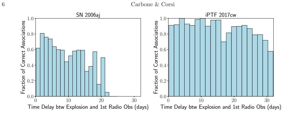
The paper's central claim is that a fixed, small number of radio epochs is enough to classify the explosion type of radio-emitting stripped-envelope SNe, provided the first observation is early and the cadence is chosen by simulation rather than by habit. With the sensitivity of a two-hour VLA observation, five epochs at delays of 2, 8, 18, and 30 days after the first detection identify $97\%$ of the detectable relativistic (engine-driven) targets at $z=0.01$, while avoiding confusion with CSM-interacting supernovae and off-axis GRBs; at $z=0.1$ the same strategy identifies $78\%$ of detectable targets. For CSM-interacting SNe, a low-urgency first observation plus delays of about 6 and 90 days classifies all detectable simulated sources. For off-axis GRBs, five epochs with a high-urgency start give $99\%$ efficiency at $z=0.01$ for detectable sources. The paper also reports a new VLA upper limit on the late-time radio emission of iPTF 17cw and projects X-ray detectability under a synchrotron radio-to-X-ray extrapolation.
Load-bearing premise
All efficiencies rest on the template light curves being representative of the true stripped-envelope supernova population; where early-time data are missing, early rises are borrowed from other SNe, so a real event that rises or fades outside the template range could break the optimized cadence.
Editorial extensions
If this is right
- A relativistic supernova needs its first radio observation within roughly 1 hour to 2 days of optical discovery; waiting a week or more lowers the identifiable fraction noticeably.
- The five-epoch campaign for relativistic SNe at $z=0.01$ costs about ten hours of VLA time per target, so a season of follow-up can cover a sizable sample rather than one or two objects.
- For CSM-interacting SNe the cadence is much slower: a first observation followed by delays near 6 and 90 days identifies every detectable simulated source, so these events do not force an urgent telescope response.
- Off-axis GRB afterglows with isotropic energy above $10^{51}$ erg are detected and uniquely identified near 100% of the time at $z=0.01$, while low-energy models below $10^{49}$ erg are mostly undetectable.
- If the radio-to-X-ray spectral index is about 0.7, Chandra-class 20 ks exposures should see the X-ray counterparts of nearby ($z=0.01$) relativistic and CSM-interacting SNe for hundreds of days.
Reading between the lines
- Inference: The same optimization machinery could be re-run for a next-generation array with roughly ten times the VLA sensitivity; the paper notes such an instrument would reach about three times farther and increase detections by a factor of order thirty, but it does not simulate its optimal cadence.
- Inference: Because the recommended epochs are derived from a small set of bright historical events, the 2-8-18-30-day pattern should be read as a starting point rather than a law; the paper's own early-time extrapolation exercise shows how much the cadence moves when the rising part of the light curve is filled in.
- Inference: Joint radio-X-ray scheduling is a natural extension of the paper's approach; a single campaign that picks radio epochs while also predicting X-ray visibility could break the degeneracy between environment density and the fraction of shock energy in magnetic fields.
Signed reviews
Editorial analysis
A structured set of objections, weighed in public.
Referee Report
Summary. The paper presents a Monte Carlo simulation framework to optimize radio follow-up observations of stripped-envelope core-collapse SNe with the VLA. The authors simulate light curves from template radio observations of known relativistic SNe (SN 1998bw, SN 2006aj, SN 2009bb, iPTF17cw), CSM-interacting SNe (PTF11qcj, SN2007bg), and BOXFIT models of off-axis GRBs, then determine the minimum number and timing of radio epochs that maximize the fraction of unique and correct associations between an observed target and its generating template. For relativistic SNe at z=0.01, they report that five observations at approximately 2, 8, 18, and 30 days after the first radio observation yield 97% efficiency. They also present a new late-time VLA upper limit on iPTF17cw and estimate X-ray detectability of the same sources. The paper includes a discussion of the importance of early-time observations and of the limited CSM-interacting sample.
Significance. If the reported efficiencies were robust, the proposed cadence would be a practical guideline for upcoming transient surveys (ZTF, LSST) and for VLA/ngVLA follow-up, using only 5 epochs. The simulation strategy is transparent, uses large Monte Carlo sets (10,000 realizations), and the authors explicitly test the effect of early-time extrapolations. The new upper limit on iPTF17cw is a modest but useful observational contribution. However, the central quantitative claims are currently based on in-sample template retrieval, which means the headline efficiencies are likely upper bounds. With a leave-one-out validation or appropriately softened claims, the paper would offer a useful planning tool, but in its present form the significance of the specific numbers is unclear.
major comments (3)
- [Section 3.3, Table 2] The definition of a 'correct' association is that the unique matching template is 'the same template/model from which the observations were simulated' (Section 3.3). Since the simulated light curves are generated from the same templates that form the classification bank, every simulated event is, by construction, a member of the bank. The reported efficiencies (Table 2, e.g., 97% at z=0.01) are therefore retrieval rates from a closed set of known templates, not classification rates for real events. A real stripped-envelope SN with a light curve that is not well represented by one of the four relativistic templates (or two CSM templates) could be uniquely matched to a wrong template, and such failures are absent from the simulation. I recommend either (a) a leave-one-out test in which each template is excluded from the bank and then used to generate simulated targets, or (b) an explicit statement that the quoted efficiencies are conditional on the template bank being representative of the true population, and should be regarded as upper bounds. This point is load-bearing because the paper's abstract and conclusions present these efficiencies as the basis for the proposed follow-up cadence.
- [Section 3.1, Table 1] The relativistic SN template bank comprises only SN 1998bw, SN 2006aj, SN 2009bb, and iPTF17cw. These are extreme events: two are very bright nearby explosions, one is very faint and rapidly fading, and one is at higher redshift with sparse early-time sampling. The simulation assumes linear interpolation/extrapolation of fluxes (Section 3.1), including extrapolation of early-time behavior from other SNe in Section 4.1.1, but there is no test of how the optimized epochs perform for light curves with, e.g., intermediate peak luminosities, different rise times, or different spectral indices. The CSM-interacting class is even more limited (only PTF11qcj and SN2007bg; the authors acknowledge this in Section 4.2). Because the proposed cadence (Table 2) is selected to maximize discrimination among these specific templates, it may not generalize to the broader stripped-envelope SN population. I would like to see a sensitivity study with perturbed template shapes (e.g., varying peak luminosity, rise time, decay rate) to demonstrate that the optimized cadence is not tailored to the individual events.
- [Section 3.3] The epoch-selection procedure optimizes the delays M2, M3, ... by maximizing the number of unique and correct associations computed on the same Monte Carlo realizations that are later used to evaluate the strategy. There is no separation between the data used to choose the epochs and the data used to measure the efficiency; thus the reported percentages are in-sample and expected to be optimistically biased. A cross-validation approach, in which the 10000 realizations are split into a training set for epoch selection and a test set for evaluation, would quantify the degree of optimism. Without this, the reader cannot tell how much of the 97% is a genuine property of the cadence and how much is overfitting to the particular realizations and templates.
minor comments (6)
- [Table 1] There is a typo in the reference line for SN 2009bb: 'Strauss et al. (1992) anf Soderberg et al. (2010)' should read 'and'.
- [Figure 2] The caption contains the typo 'campiagn'; it should be 'campaign'.
- [Sections 2 and 4] The source is referred to inconsistently as both 'iPTF17cw' and 'PTF 2017cw'; the standard naming 'iPTF 17cw' should be used throughout.
- [Section 3.3] The notation for time delays is not fully consistent: the text defines 'Delta Tn = tn - tradio,0 = Mn x 2 d' but later uses 'Delta t2 = M2 x 2 d' and 'Delta t3'; harmonize the notation for readability.
- [Section 5, Eq. (1)] The spectral index convention F_nu proportional to nu^{-beta} is stated earlier for SN 2006aj but not near Eq. (1); it should be explicitly restated when the radio-to-X-ray spectral index is introduced.
- [Sections 4.1-4.3] The efficiencies are computed after excluding non-detectable targets, which is a reasonable choice; however, it would also be informative to report the absolute fraction of all simulated targets that are correctly associated (including non-detections), since in a real follow-up one does not know detectability a priori.
Circularity Check
In-sample template retrieval: the reported 97% efficiency is the objective used to choose the optimized epochs, not an out-of-sample prediction.
-
fitted input called prediction
[Section 3.3 (Monte Carlo optimization); Table 2 in Section 4.1]
"Thus, we optimize the value of M2 by maximizing the number of associations that in epoch two become unique (only one model/template fits the observed target in both epochs) and correct (the model/template that fits the observations uniquely is also the correct one, i.e. it is the same template/model from which the observations were simulated)."
Correctness is defined, by construction, as recovering the exact template that generated the simulated light curve. The same 10,000 simulated realizations are used both to fit the epoch delays (maximizing the number of unique+correct associations) and to compute the efficiency reported in Table 2. The 97% figure is therefore the in-sample training objective, not a held-out accuracy: it quantifies how well the chosen cadence separates the four specific relativistic SN templates from the contaminants under the assumed noise, and any real stripped-envelope SN not represented by these templates is outside the evaluation. The cadence recommendation may still be useful, but the headline efficiency is inflated by construction and should be read as an upper bound.
full rationale
The paper's central derivation is a Monte Carlo optimization: it generates simulated light curves from template radio light curves, chooses follow-up epochs to maximize unique+correct associations, and reports the resulting efficiency. The one significant circular step is that the efficiency is evaluated on the same simulated data used to fit the epochs, with 'correct' defined as identity with the generating template. This makes the 97% (z=0.01) and related efficiencies in-sample retrieval scores rather than out-of-sample predictions. No load-bearing self-citation or imported uniqueness theorem occurs: Carbone & Corsi (2018) is cited only as the methodological predecessor and the method is fully restated; the iPTF17cw data are observational. The physical timing conclusions (early radio observations for relativistic SNe, later for CSM-interacting SNe) are independently motivated by the shapes of the observed light curves and remain plausible, so the circularity is partial, not total. The paper is transparent about its small template sample, but the headline association rates should be labeled as training-set accuracy or validated with a held-out set of light-curve shapes.
Assumptions & free parameters
free parameters (7)
- Eiso of off-axis GRB models =
1e48 to 1e54 erg
- Viewing angle theta_v =
24 deg and 45 deg
- Afterglow microphysics (eps_B, eps_E, p, theta_j, n_ISM) =
1e-2, 1e-1, 2.5, 12 deg, 1 cm^-3
- VLA observation RMS sigma_obs =
5 uJy at 5 GHz
- Detection threshold =
3 sigma = 15 uJy
- Epoch grid step =
2 days
- Maximum number of epochs =
10
assumptions (5)
- domain assumption BOXFIT v2 standard fireball afterglow model describes off-axis GRB radio emission.
- ad hoc to paper The six observed SN light curves are representative of the stripped-envelope SN population.
- domain assumption The set of contaminants (relativistic SNe, CSM-interacting SNe, off-axis GRBs) is complete.
- ad hoc to paper Linear interpolation and extrapolation of template fluxes is valid at simulated epochs.
- domain assumption The radio-to-X-ray spectrum is a single power law with beta 0.7-1 (Eq. 1).
Cite this review
Pith. "Pith review of An optimized radio follow-up strategy for stripped-envelope core-collapse supernovae." pith.science (2026). https://pith.science/paper/CZHZCYWE
@misc{pith2026190806190,
  author       = {Pith},
  title        = {Pith review of: An optimized radio follow-up strategy for stripped-envelope core-collapse supernovae},
  year         = {2026},
  howpublished = {\url{https://pith.science/paper/CZHZCYWE}},
  note         = {Machine review of arXiv:1908.06190}
}
read the original abstract
Several on-going or planned synoptic optical surveys are offering or will soon be offering an unprecedented opportunity for discovering larger samples of the rarest types of stripped-envelope core-collapse supernovae (SNe), such as those associated with relativistic jets, mildly-relativistic ejecta, or strong interaction with the circumstellar medium (CSM). Observations at radio wavelengths are a useful tool to probe the fastest moving ejecta, as well as denser circumstellar environments, and can thus help us identify the rarest type of core-collapse explosions. Here, we discuss how to set up an efficient radio follow-up program to detect and correctly identify radio-emitting stripped-envelope core-collapse explosions. We use a method similar to the one described in \citealt{Carbone2018}, and determine the optimal timing of GHz radio observations assuming a sensitivity comparable to that of the Karl G. Jansky Very Large Array. The optimization is done so as to ensure that the collected radio observations can identify the type of explosion powering the radio counterpart by using the smallest possible amount of telescope time. We also present a previously unpublished upper-limit on the late-time radio emission from supernova iPTF17cw. Finally, we conclude by discussing implications for follow-up in the X-rays.
Figures

Reference graph
Works this paper leans on
-
[1]
Adelman-McCarthy, J. K., Ag¨ ueros, M. A., Allam, S. S., et al . 2006, ApJS, 162, 38
work page 2006
-
[2]
2006, MNRAS, 372, 233
Amati, L. 2006, MNRAS, 372, 233
2006
-
[3]
2002, A&A, 390, 81
Amati, L., Frontera, F., Tavani, M., et al. 2002, A&A, 390, 81
2002
-
[4]
Bellm, E. C. 2016, PASP, 128, 084501
2016
-
[5]
Beniamini, P., & van der Horst, A. J. 2017, MNRAS, 472, 3161
work page 2017
-
[6]
Berger, E., Kulkarni, S. R., Frail, D. A., & Soderberg, A. M. 2003, ApJ, 599, 408
work page 2003
- [7]
-
[8]
N., Hill, J
Burrows, D. N., Hill, J. E., Nousek, J. A., et al. 2005, Space Sci. Rev., 120, 165
2005
Show all 51 references
-
[9]
J., et al
Campana, S., Mangano, V., Blustin, A. J., et al. 2006, Nature , 442, 1008
2006
-
[10]
2018, ApJ, 867, 135
Carbone, D., & Corsi, A. 2018, ApJ, 867, 135
2018
-
[11]
Chandra, P., & Frail, D. A. 2012, ApJ, 746, 156
2012
-
[12]
A., & Fransson, C
Chevalier, R. A., & Fransson, C. 2006, ApJ, 651, 381
2006
-
[13]
O., Frail, D
Corsi, A., Ofek, E. O., Frail, D. A., et al. 2011, ApJ, 741, 76
2011
-
[14]
O., Gal-Yam, A., et al
Corsi, A., Ofek, E. O., Gal-Yam, A., et al. 2014, ApJ, 782, 42
2014
-
[15]
R., et al
Corsi, A., Gal-Yam, A., Kulkarni, S. R., et al. 2016, ApJ, 830 , 42
2016
-
[16]
B., Kasliwal, M
Corsi, A., Cenko, S. B., Kasliwal, M. M., et al. 2017, ApJ, 847 , 54
2017
-
[17]
1999, ApJ, 521, L117
Eichler, D., & Levinson, A. 1999, ApJ, 521, L117
1999
-
[18]
C., Berezhko, E
Ellison, D. C., Berezhko, E. G., & Baring, M. G. 2000, ApJ, 540 , 292
2000
-
[19]
Filippenko, A. V. 1997, ARA&A, 35, 309
1997
-
[20]
2006, A&A, 447, 8 91
Foley, S., W atson, D., Gorosabel, J., et al. 2006, A&A, 447, 8 91
2006
-
[21]
A., Kulkarni, S
Frail, D. A., Kulkarni, S. R., Sari, R., et al. 2001, ApJ, 562, L55
2001
-
[22]
2017, Observational and Physical Classificatio n of Supernovae, 195
Gal-Yam, A. 2017, Observational and Physical Classificatio n of Supernovae, 195
2017
-
[23]
J., Vreeswijk, P
Galama, T. J., Vreeswijk, P. M., van Paradijs, J., et al. 1998 , Nature, 395, 670
1998
-
[24]
2004, ApJ, 61 1, 1005
Gehrels, N., Chincarini, G., Giommi, P., et al. 2004, ApJ, 61 1, 1005
2004
-
[25]
2005, MNRAS, 36 1, L10
Ghirlanda, G., Ghisellini, G., & Firmani, C. 2005, MNRAS, 36 1, L10
2005
-
[26]
2004, ApJ, 616, 331
Ghirlanda, G., Ghisellini, G., & Lazzati, D. 2004, ApJ, 616, 331
2004
-
[27]
J., Kulkarni, S
Graham, M. J., Kulkarni, S. R., Bellm, E. C., et al. 2019, PASP , 131, 078001
2019
-
[28]
Granot, J., & van der Horst, A. J. 2014, PASA, 31, e008
2014
-
[29]
Ho, A. Y. Q., Goldstein, D. A., Schulze, S., et al. 2019, arXiv e-prints, arXiv:1904.11009
2019 arXiv
-
[30]
Kellermann, K. I. 1964, ApJ, 140, 969
1964
-
[31]
R., Frail, D
Kulkarni, S. R., Frail, D. A., Wieringa, M. H., et al. 1998, Na ture, 395, 663
1998
-
[32]
M., Kulkarni, S
Law, N. M., Kulkarni, S. R., Dekany, R. G., et al. 2009, PASP, 121, 1395 LSST Science Collaboration, Abell, P. A., Allison, J., et al . 2009, arXiv e-prints, arXiv:0912.0201
2009 arXiv
-
[33]
D., Chornock, R., et al
Margutti, R., Metzger, B. D., Chornock, R., et al. 2019, ApJ, 872, 18
2019
-
[34]
2014, MNRAS, 443, 67
Tanaka, M. 2014, MNRAS, 443, 67
2014
-
[35]
P., W aters, B., Schiebel, D., Young, W., & Golap , K
McMullin, J. P., W aters, B., Schiebel, D., Young, W., & Golap , K. 2007, in Astronomical Society of the Pacific Conference
2007
-
[36]
J., Bolatto, A., Chatterjee, S., et al
Murphy, E. J., Bolatto, A., Chatterjee, S., et al. 2018, in Astronomical Society of the Pacific Conference Series, Vol. 517, Science with a Next Generation Very Large Array, ed. E. Murphy, 3
2018
-
[37]
2012, MNRAS, 421, 1256
Nava, L., Salvaterra, R., Ghirlanda, G., et al. 2012, MNRAS, 421, 1256
2012
-
[38]
T., Corsi, A., Frail, D
Palliyaguru, N. T., Corsi, A., Frail, D. A., et al. 2019, ApJ, 872, 201
2019
-
[39]
A., Cenko, S
Perley, D. A., Cenko, S. B., Corsi, A., et al. 2014, ApJ, 781, 3 7
2014
-
[40]
1998, ApJ, 509, L85
Perna, R., & Loeb, A. 1998, ApJ, 509, L85
1998
-
[41]
2004, Reviews of Modern Physics, 76, 1143
Piran, T. 2004, Reviews of Modern Physics, 76, 1143
2004
-
[42]
J., Maguire, K., Smartt, S
Prentice, S. J., Maguire, K., Smartt, S. J., et al. 2018, ApJ, 865, L3
2018
-
[43]
Rhoads, J. E. 1997, ApJ, 487, L1
1997
-
[44]
E., Stockdale, C., & Prieto, J
Salas, P., Bauer, F. E., Stockdale, C., & Prieto, J. L. 2013, MNRAS, 428, 1207
2013
-
[45]
2017, PASP, 129, 054201
Shivvers, I., Modjaz, M., Zheng, W., et al. 2017, PASP, 129, 054201
2017
-
[46]
M., Dekany, R
Smith, R. M., Dekany, R. G., Bebek, C., et al. 2014, in Proc. SPIE, Vol. 9147, Ground-based and Airborne Instrumentation for Astronomy V, 914779 Optimized radio follow-up strategy for rare Ib/c SNe 9
2014
-
[47]
M., Chakraborti, S., Pignata, G., et al
Soderberg, A. M., Chakraborti, S., Pignata, G., et al. 2010, Nature, 463, 513
2010
-
[48]
O., Fynbo, J
Sollerman, J., Jaunsen, A. O., Fynbo, J. P. U., et al. 2006, A& A, 454, 503
2006
-
[49]
A., Huchra, J
Strauss, M. A., Huchra, J. P., Davis, M., et al. 1992, ApJS, 83 , 29 van Eerten, H., van der Horst, A., & MacFadyen, A. 2012, ApJ, 749, 44
1992
-
[50]
2017, X-Ray Emission Properties of Supernova Remnants, ed
Vink, J. 2017, X-Ray Emission Properties of Supernova Remnants, ed. A. W. Alsabti & P. Murdin, 2063 W axman, E. 2004, ApJ, 602, 886 W oosley, S. E., & Bloom, J. S. 2006, ARA&A, 44, 507
2017
-
[51]
2003, ApJ, 594, L7 9
Yamazaki, R., Yonetoku, D., & Nakamura, T. 2003, ApJ, 594, L7 9
2003
Reviewed August 14, 2026 · model on record in the stance chip above.
Discussion (0). Continue with ORCID to comment.