Renormalizable Graph Embeddings For Multi-Scale Network Reconstruction

Diego Garlaschelli; Fabian Jansen; Riccardo Milocco

REVIEW 3 major objections 4 minor 67 references

Renormalizable Graph Embeddings For Multi-Scale Network Reconstruction

T0 review · 3 major / 4 minor · reviewed 2026-08-05 · deepseek-v4-flash

Challenge this review Re-run · record.json Download PDF Read on arXiv ↗ Review JSON

Pith's one-line read Scale-invariant multi-scale models yield graph embeddings that stay consistent under node aggregation, so one fit at the finest scale predicts links at every coarser scale, while maximum-entropy models must be refitted each level.

desk verdict The additive renormalization is mathematically sound and the comparison is honest, but the paper sells a model-internal identity as empirical support, so the strongest claims need to be dialed back. read the letter →

arxiv 2508.20706 v1 pith:D4NZZVPG submitted 2025-08-28 physics.soc-ph cond-mat.dis-nnecon.GNq-fin.EC

Riccardo Milocco , Fabian Jansen , Diego Garlaschelli This is my paper · ORCID

classification physics.soc-phcond-mat.dis-nnecon.GNq-fin.EC PACS 89.65.Gh89.75.-k

keywords multi-scalenetworkreconstructiongraphembeddingsscaleinvariancerenormalizationconfigurationmodelmaximumentropyinput-outputnetworksworldtradeweb

verification ladder T0 review T1 audit T2 compute T3 formal

The pith

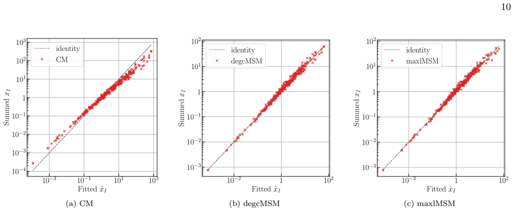
A machine-rendered reading of the paper's core claim, the machinery that carries it, and where it could break.

The reading

This paper asks how to reconstruct a hidden network from partial or aggregate data when the resolution of the data changes because nodes are grouped into blocks, as happens when firms are aggregated into sectors or countries into trade regions. It argues that the standard maximum-entropy reconstruction models—the configuration model (CM) and its fitness-based variant (fitnCM)—are single-scale: their parameters are only meaningful at the level where they were fitted and must be re-estimated at every other level. The proposed alternative, the multi-scale model (MSM) family derived from the principle of scale invariance, keeps the same functional form at every resolution and renormalizes block parameters by simply summing the microscopic ones. If the paper is right, a model fitted once at the finest observable scale predicts connection probabilities at all coarser scales without refitting, and node embedding vectors transform additively under aggregation. On a confidential national input-output network and on the World Trade Web, the degree-corrected MSM matches or beats the configuration model, including at the level where both models are fitted, while the fitness-based MSM reproduces the total number of links at every scale.

What carries the argument

The load-bearing identity is the scale-invariance condition of Equation 19: the renormalized (summed) probability of a block-edge must equal the coarse-grained probability that at least one microscopic edge is present, with both expressed in the same functional form. The unique functional form compatible with this constraint under the independent-edge assumption is the MSM link probability p_ij = 1 − e^{−x_i x_j} (plus a self-loop term), which in turn yields the additive renormalization rule x_I = Σ_{i∈I} x_i, w_I = Σ_{i∈I} w_i (Equation 20). This sum rule is the mechanism that carries the argument: it makes node parameters additive under aggregation, and it guarantees that a single fit at l

What would settle it

Fit the MSM at the finest level of a network with strong community structure or correlated edges, sum the parameters to a coarser level, and compare predicted block-edge probabilities with the observed coarsened network. If the empirical fraction of linked block pairs falls systematically outside the model's Bernoulli prediction intervals, the scale-invariance is an algebraic identity of the model rather than a property of the data. The paper's own finding that fitnCM beats fitnMSM where the fitness proxy is weak offers the complementary check: a dataset where the refitted single-scale model b

Watch

Extended reading notes

Core claim

The central claim is that the multi-scale model (MSM), with connection probability p_ij = 1 − e^{−x_i x_j} and a matching self-loop term, is the functional form satisfying scale invariance under logical-OR node aggregation: the probability that two blocks are linked equals the probability that at least one edge exists between their members, in the same functional form at every level. Consequently block parameters renormalize by summation, x_I = Σ_{i∈I} x_i and w_I = Σ_{i∈I} w_i, so the embeddings are additive under coarse-graining and never re-learned. The configuration model p_ij = x_i x_j/(1 + x_i x_j) is not renormalizable: coarse-graining its probabilities yields a function outside the C

Load-bearing premise

The whole construction assumes the real network is generated by independent edges combined with logical-OR aggregation—a block is linked if at least one of its members is linked—so that the model's additive summation rule mirrors the true coarse-graining; if real edges are correlated or aggregation works differently, the 'consistent embeddings' are a property of the model, not of the data.

Editorial extensions

If this is right

A model fitted once at the finest observable scale applies to any coarser representation, so no refitting is needed when the data resolution changes.
Node embedding vectors become additive under aggregation, giving a principled interpretation to vector sums in latent space and connecting embeddings across resolutions.
The degree-corrected MSM outperforms the configuration model at the fitted level 0 and keeps high reconstruction accuracy for degrees, nearest-neighbour degree, and clustering at coarser levels.
The fitness-based MSM needs only additively aggregating exogenous variables (strengths or GDP) and preserves the total number of links at every scale, which matters when degrees are confidential.
Renormalizing by summation instead of coarse-graining microscopic probabilities cuts the computational cost by roughly (N_ℓ/N_0)² at level ℓ.

Reading between the lines

Editorial extensions of the paper, not claims the author makes directly.

The consistency is algebraic once the independent-edge, OR-aggregation generating process is assumed; whether real supply and trade networks obey it is an empirical question the paper does not settle. A direct test would compare the distribution of edge counts between blocks in observed data with the Bernoulli prediction.
The additive sum rule suggests a screening principle: any latent-space model whose link function satisfies the coarse-graining identity inherits renormalizability, so other functional forms could be tested for this property rather than derived from first principles.
The paper's own result that fitnCM beats fitnMSM wherever the fitness proxy is weak implies a practical hybrid: use degree constraints where available and additively consistent fitness constraints where privacy forbids them, since the MSM's sum rule keeps mixed constraints consistent across scales.
Because the paper's interlude (Section V B 1) warns that metric-level agreement between summed and refitted models should not be read as scale invariance, the practical advantage of MSMs should be evaluated with the identity of Equation B8, not just with reconstruction scores.

Share X Bluesky LinkedIn Reddit HN

Signed reviews

No signed human review yet.

Editorial analysis

A structured set of objections, weighed in public.

Desk editor's note, referee report, and a circularity audit.

Desk Editor's Note

read the letter

The paper's new pieces are the degree-corrected and maximum-likelihood MSMs (degcMSM, maxlMSM), the renormalized single-scale variants, and the two empirical applications on the ING bank data and the World Trade Web. The core mathematics is in good shape: the additive renormalization rule follows directly from the model's independent-edge, logical-OR structure, and the proof that the Configuration Model is not scale-invariant (Appendix A1) is clean and correct. The authors also deserve credit for releasing code, using publicly available WTW data, and reporting mixed results without hiding them—e.g., fitnCM beats fitnMSM on AUC/PR, which is not what a partisan author would highlight.

The soft spots are real but not fatal. Figure 2 is presented as evidence for scale invariance, yet it is a tautology: summed probabilities equal coarse-grained probabilities because the model was constructed that way. The paper actually acknowledges this in Section V B 1, which is good, but the Conclusions still say the MSM is "aligning with the hidden generative process." That is overreach. The framework assumes the true micro network is MSM-distributed and that aggregation is logical OR; this is an imposed modeling assumption, and the paper never tests it against the data. If real firm or trade networks violate that form, the nice additive rule is just an algebraic identity, not a discovered property of the system.

The empirical comparisons also need more caution. The claim that degcMSM outperforms CM at the fitted level rests on one confidential dataset with no error bars or significance tests. The RA metric has dispersion intervals, but the AUC and PR comparisons are point estimates with no uncertainty. On the WTW, the fitness ansatz is weak by the paper's own analysis, so the fitness-model results are less informative. These are fixable issues: report bootstrap or repeated-sampling uncertainty, and soften the language about the hidden generative process.

Who is this for? People doing network reconstruction, especially for systemic-risk applications, and anyone working on multi-scale or renormalizable graph models. The theoretical contribution is worth their time, and the benchmark comparison, despite the caveats, is a useful data point. I would send this to peer review—it deserves a serious referee—but with clear requests: quantify uncertainty, test the model assumptions on data where possible, and separate the built-in consistency of the MSM from empirical validation.

In short: the math is sound, the paper is honest, and the new model variants are useful, but the rhetoric about alignment with the true generative process should be tempered.

Referee Report

3 major / 4 minor

Summary. The paper develops graph-embedding methods for network reconstruction in a multi-resolution setting. It contrasts maximum-entropy single-scale models (CM, fitnCM) with scale-invariant multi-scale models (degcMSM, maxlMSM, fitnMSM), where block-level parameters are defined as sums of microscopic parameters and link probabilities take the MSM form p_ij = 1 - exp(-x_i x_j). The central mathematical claim is that this form is renormalizable under arbitrary node aggregation: the coarse-grained probability is exactly the MSM probability with summed parameters. The paper tests the methods on an ING input-output network at several NAICS aggregation levels and on the WTW, reporting scale-invariance plots, parameter agreement, signed relative errors of link counts, reconstruction accuracies, AUC-ROC/PR curves, and triangle-density comparisons. The claimed payoffs are that a model fitted once at the finest resolution predicts coarser scales consistently, and that degcMSM improves over CM even at the fitted level.

Significance. The additive renormalization rule for the MSM is mathematically correct and potentially useful: it gives an interpretable, parameter-free transformation of node embeddings under aggregation. The paper is also transparent about the model assumptions and releases code. However, the main empirical support for the practical claim is currently weak: the headline scale-invariance check is an identity by construction, and the comparative results are point estimates without uncertainty quantification. If the model were tested against non-MSM generative processes and with proper significance analysis, the contribution would be solid. As it stands, the theoretical part is sound but the empirical validation of the central claim is incomplete.

major comments (3)

[Section V A, Appendix B (Eqs. B5–B8), Fig. 2] The scale-invariance evidence in Fig. 2 is a model-internal identity, not an empirical test. Eq. (B8) is derived by assuming independent edges p=1-exp(-x_i x_j), OR aggregation, and summed parameters; it holds by construction for any fitted MSM parameters. The text itself says 'By construction' in Section V A, and Section V B 1 restricts 'true' scale-invariance to Eq. B8. Yet the Conclusion (Section VI) claims MSMs 'align with the hidden generative process.' This overstates what is demonstrated. Please add a falsifiable test, e.g. apply the same identity to synthetic networks generated by a non-MSM model, compare level-l likelihoods of summed MSM versus refitted alternatives, or show how deviations from the independent-edge/OR assumption would be detected. Without this, the central claim that a model fitted once predicts coarser scales rests on an imposed assumption.
[Section V F–G, Figs. 5, 7a, 7b] The quantitative comparisons that support the paper's empirical claims are reported without error bars or significance tests. For instance, Fig. 5 reports signed relative errors as single curves; Fig. 7a reports reconstruction accuracies without dispersion; Fig. 7b reports AUC curves without bootstrap intervals. Section V G explicitly acknowledges that 'it remains difficult to differentiate single-scale from multi-scale models, as their AUC performances are often coinciding,' and that fitnCM consistently outperforms fitnMSM. Given that each dataset is a single realization, please provide uncertainty quantification (e.g., bootstrap over nodes/edges or over repeated random partitions) and state which differences are statistically significant. The current wording (e.g., 'degcMSM delivers the best performance at the fitted level') is stronger than the evidence supports.
[Abstract / Introduction vs. Section V] The paper motivates the problem as reconstructing an unobserved microscopic network from aggregate information (e.g., firm-level links hidden behind sector-level data). However, all experiments fit the models at the finest available level (level 0) and then aggregate upward; there is no experiment where the micro network is withheld and inferred from coarse data. Thus the privacy-oriented reconstruction direction promised in the abstract is not actually evaluated. A proof-of-concept in the reverse direction—or a revision of the framing—is needed, because the practical relevance of the additive sum rule to the stated problem depends on that direction.

minor comments (4)

[Section III C 2 vs. Appendix B 2 b] The main text states that at the optimum of maxlMSM, nodes with identical neighbors have the same parameters, but Appendix B 2 b says the stationarity condition does not guarantee this and that statistical equivalence is imposed by hand. Please reconcile these statements.
[Appendix B 2 a, Eqs. (B10)–(B12)] The claimed stationary solution for w_i is not a stationary point of the likelihood: for a_ii=0 the derivative is identically -1, and for a_ii=1 the derivative 1/p_ii-1 vanishes only in the limit w_i→∞. These are boundary/limit solutions, not solutions of ∂_{w_i} L=0. Clarify the formulation.
[Section V G, Fig. 7 caption] The caption says 'for the fitted models (level 0) and summed ones (level 2)' but the axes show all levels 0–3; update the wording. Also fix the typo 'Novertheless' in Section V G.
[Section V B 1] The statement that 'true deviation from scale-invariance should be only assessed using Eq. (B8)' is circular given that Eq. (B8) is an identity of the model. The sentence should be rewritten to acknowledge that Eq. (B8) tests internal consistency, not empirical validity.

Circularity Check

2 steps flagged · score 4.0 of 10

The scale-invariance 'evidence' is an algebraic identity of the MSM, but the multi-scale reconstruction predictions are genuine out-of-sample and mostly self-contained.

self definitional [Section V A (Figure 2)]
"Figure 2 illustrates the property of scale-invariance by plotting the left-hand side (LHS) of the equation in Equation B8 against its right-hand side (RHS). By construction, both the fitnMSM and degcMSM models perfectly recover the identity line, while the maxlMSM is not depicted since it uses the same probability as the degcMSM."

Equation B8 is the defining identity of the MSM: for p(xi,xj)=1-exp(-xi*xj), the coarse-grained probability 1-prod(1-p) equals 1-exp(-(sum xi)(sum xj)), which is exactly the MSM probability evaluated at summed parameters. Therefore the plotted identity line is an algebraic identity of the model, not an empirical test that the data are scale-invariant. The text explicitly says 'by construction'; presenting this as 'Scale-Invariance Evidence' turns the model definition into purported evidence.
self definitional [Section V B 1]
"Therefore, true deviation from scale-invariance should be only assessed using the Equation B8 shown in Figure 2, since other metrics can lead to misleading results that depend on the specific scale or quantity."

The paper first acknowledges that scale-invariance does not imply that summed and refitted predictions agree, then directs evaluation exclusively to Equation B8. For the MSM, Equation B8 is satisfied by construction for any parameter values and cannot fail; hence it cannot assess 'true deviation from scale-invariance' in real data. This validation step reduces to checking the model's own definition rather than testing its empirical adequacy.

full rationale

The central mathematical construction—block parameters as sums of microscopic parameters—is an intentional design property of the MSM and is presented as such, not hidden. The paper's actual empirical claims (link counts, degrees, clustering, reconstruction accuracies at coarser levels using level-0 fitted parameters) are genuine out-of-sample predictions and are not circular: they are computed from parameters fitted at level 0 and compared to data at higher levels. The acknowledged circularity is limited to the 'Scale-Invariance Evidence' of Figure 2, which is an algebraic identity of the MSM, and to the subsequent recommendation to judge scale-invariance by that tautological equation. The paper also relies on prior work by the same group ([13], [18]) for the uniqueness and functional form of the MSM, but Appendix B re-derives the key identity, so the self-citations are not the sole load-bearing support. The mixed empirical results (e.g., fitnCM outperforming fitnMSM on several metrics, AUC scores often indistinguishable) are independent checks rather than circular arguments. Lack of error bars is a robustness concern, not circularity. Overall, the core derivation is mostly self-contained, but because one of the paper's validation exhibits reduces by construction to the model definition, a moderate circularity score is warranted.

Assumptions & free parameters 3 free parameters · 5 assumptions · 0 invented entities

The model class borrows the MSM framework and sum rule from prior papers [13,18] by the same group. The paper's new contributions are estimation variants (degcMSM, maxlMSM), renormalized versions of CM and fitnCM, and the empirical comparison. Free parameters are the per-node propensities x_i, the self-loop terms w_i, and the global delta in fitness models. No new physical entities are introduced.

free parameters (3)

x_i (node propensities) = fitted at level 0 to degrees/likelihood
For CM, one value per unique degree; for degcMSM one per node; for maxlMSM one per structurally equivalent class. Summed to block parameters via Eq. 20.
w_i (MSM self-loop propensities) = boundary values in maxlMSM; unspecified for degcMSM
Appear in Eq. 12 for self-loops; the paper discards self-loops in comparisons, but w_I appears in the summed self-loop probability.
delta (global coupling) = fixed at level 0 via total link count L
Single global parameter in fitnCM/fitnMSM; method of moments, Eq. 18.

assumptions (5)

domain assumption Edges are independent Bernoulli variables with probability p_ij (Eq. 5)
All models treat each pair independently; this ignores higher-order dependencies present in real networks.
ad hoc to paper Scale invariance: the same functional form must hold at every resolution and renormalized block probabilities must equal coarse-grained microscopic probabilities (Eq. 19/B8)
This is the defining principle of the MSM family, imposed rather than derived from data.
domain assumption Fitness ansatz: x_i proportional to sqrt(delta) * phi_i with observed fitness phi_i (Eq. 9)
Assumes node propensities are fully explained by strengths (ION) or GDP (WTW); the paper shows this is a weak approximation for WTW (Fig. 13 caption).
domain assumption Coarse-graining is logical OR over micro links (Eq. 1)
Block-level edges exist if at least one micro edge exists; real aggregation processes may differ.
ad hoc to paper In the MSM derivation, g(x) is chosen as the identity function 'for simplicity' (Appendix B1)
Any positive monotonic g with g(sum) = sum g would satisfy the functional equation; identity is a simplifying choice that fixes the model form.

how reviews work

0 comments

Cite this review

Pith. "Pith review of Renormalizable Graph Embeddings For Multi-Scale Network Reconstruction." pith.science (2026). https://pith.science/paper/D4NZZVPG

@misc{pith2026250820706,
  author       = {Pith},
  title        = {Pith review of: Renormalizable Graph Embeddings For Multi-Scale Network Reconstruction},
  year         = {2026},
  howpublished = {\url{https://pith.science/paper/D4NZZVPG}},
  note         = {Machine review of arXiv:2508.20706}
}

read the original abstract

In machine learning, graph embedding algorithms seek low-dimensional representations of the input network data, thereby allowing for downstream tasks on compressed encodings. Recently, within the framework of network renormalization, multi-scale embeddings that remain consistent under an arbitrary aggregation of nodes onto block-nodes, and consequently under an arbitrary change of resolution of the input network data, have been proposed. Here we investigate such multi-scale graph embeddings in the modified context where the input network is not entirely observable, due to data limitations or privacy constraints. This situation is typical for financial and economic networks, where connections between individual banks or firms are hidden due to confidentiality, and one has to probabilistically reconstruct the underlying network from aggregate information. We first consider state-of-the-art network reconstruction techniques based on the maximum-entropy principle, which is designed to operate optimally at a fixed resolution level. We then discuss the limitations of these methods when they are used as graph embeddings to yield predictions across different resolution levels. Finally, we propose their natural 'renormalizable' counterparts derived from the distinct principle of scale invariance, yielding consistent graph embeddings for multi-scale network reconstruction. We illustrate these methods on national economic input-output networks and on international trade networks, which can be naturally represented at multiple levels of industrial and geographic resolution, respectively.

Figures

Figures reproduced from arXiv: 2508.20706 by the authors.

**Figure 2.** FIG. 2. Testing the scale-invariance principle on the single [PITH_FULL_IMAGE:figures/full_fig_p009_2.png] view at source ↗

**Figure 3.** FIG. 3. Summed (y-axis) VS Fitted (x-axis) Parameters at level 2. From the left, we show the CM, degcMSM and maxlMSM. [PITH_FULL_IMAGE:figures/full_fig_p010_3.png] view at source ↗

Figures from the paper (14 more)

**Figure 4.** Figure 4: FIG. 4. Rescaled scalar parameters against the rescaled strengths at level 0 and 2. For level 0, the weights are directly learned [PITH_FULL_IMAGE:figures/full_fig_p010_4.png]

**Figure 5.** Figure 5: FIG. 5. Evolution of the signed relative error accross scales. [PITH_FULL_IMAGE:figures/full_fig_p011_5.png]

**Figure 6.** Figure 6: FIG. 6. Multi-Scale comparison of the Configuration Model and degree-corrected Multi Scale Model. Both have been fitted at [PITH_FULL_IMAGE:figures/full_fig_p013_6.png]

**Figure 7.** Figure 7: FIG. 7. Comparison of the PR curves for the degcMSM at scale 0, where the parameters are fitted, and level 2, with summed [PITH_FULL_IMAGE:figures/full_fig_p015_7.png]

**Figure 8.** Figure 8: FIG. 8. Comparison of the triangle density on the subgraph obtained by filtering the nodes with a lower degree tha [PITH_FULL_IMAGE:figures/full_fig_p015_8.png]

**Figure 9.** Figure 9: FIG. 9. Simple multi-scale network: the blue nodes belong to block [PITH_FULL_IMAGE:figures/full_fig_p019_9.png]

**Figure 10.** Figure 10: FIG. 10. External Structural Equivalence example: node 1 and 2 are, respectively, equivalent to node 3 and 4, even thought [PITH_FULL_IMAGE:figures/full_fig_p023_10.png]

**Figure 11.** Figure 11: FIG. 11. Plot of [PITH_FULL_IMAGE:figures/full_fig_p025_11.png]

**Figure 12.** Figure 12: FIG. 12. Summed (y-axis) VS Fitted (x-axis) Parameters at level 4. From the left, we show the CM, degcMSM and maxlMSM. [PITH_FULL_IMAGE:figures/full_fig_p029_12.png]

**Figure 13.** Figure 13: FIG. 13. Rescaled scalar parameters against the rescaled GDPs at level 0 and 2. For level 0, the weights are directly learned [PITH_FULL_IMAGE:figures/full_fig_p030_13.png]

**Figure 14.** Figure 14: FIG. 14. Evolution of the signed relative error accross scales. The error vanishes for level 0, where the models have been fitted. [PITH_FULL_IMAGE:figures/full_fig_p031_14.png]

**Figure 15.** Figure 15: FIG. 15. Multi-Scale comparison of the Configuration Model and degree-corrected Multi Scale Model. Both have been fitted at [PITH_FULL_IMAGE:figures/full_fig_p032_15.png]

**Figure 16.** Figure 16: FIG. 16. Reconstruction Accuracies of DEG, ANND and CC for all the models and levels. The models are fitted at level 0, [PITH_FULL_IMAGE:figures/full_fig_p033_16.png]

**Figure 17.** Figure 17: FIG. 17. Comparison of the triangle density on the subgraph obtained by filtering the nodes with a lower degree tha [PITH_FULL_IMAGE:figures/full_fig_p034_17.png]

Discussion (0). Continue with ORCID to comment.

Reference graph

Works this paper leans on

67 extracted references · 59 canonical work pages

[1]

They require that the renormalized probability P(ℓ) sum equals the coarse-grained P(ℓ) cog with the same functional form ([18], section B 1) for all the scales

Summed MSM This class of models is defined by enforcing the follow- ing two conditions, namely    P(ℓ) sum ! = P(ℓ) cog P(ℓ) ! ≡ P(m) (19) ∀ℓ ≥ 0, m ≥ 0, which are jointly referred to as the scale-invariance (or self-consistency) properties. They require that the renormalized probability P(ℓ) sum equals the coarse-grained P(ℓ) cog with the same functio...

work page
[2]

coarse-graining

Summed CM Once the microscopic ⃗ x(0) := {xi0 }i0∈[1,N0] have been estimated, the Configuration Model (CM) lacks a built-in renormalization procedure. As such, two possible strate- gies can be followed: “coarse-graining” the microscopic probabilities (Equation B6) or by refitting the parame- ters at that level ℓ. Both solutions suffer from a similar drawb...

work page
[3]

Public Admin- istration

Fixed (renormalized) fitnCM Similarly to the CM, the fitnCM lacks scale-invariance properties. Therefore, we implement a renormalization scheme whereby δ(ℓ) ! = δ(0) (the latter parameter was fixed at the microscopic level 0), while the block-fitness I is obtained by summing the inner fitness {ϕi}{i∈I} (see section A). Note that this approach is equivalen...

work page 2022
[4]

This does not guarantee that the predictions derived from a summed model will match those from a re-fitted one

Interlude: Scale-Invariance Implications The principle of scale-invariance, as defined in Equa- tion B5, requires that the network ensembles generated from summed and coarse-grained probabilities are sta- tistically equivalent. This does not guarantee that the predictions derived from a summed model will match those from a re-fitted one. Therefore, true d...

work page
[5]

As a result, the fitnCM is expected to yield better local-level predictions compared to the MSMs (refer to 7a)

Level 0 At level 0 (see 4a), node strengths closely approximate the parameters of the Configuration Model (CM), while they tend to underestimate those of the MSMs, especially for nodes with low values. As a result, the fitnCM is expected to yield better local-level predictions compared to the MSMs (refer to 7a). As described in section III, CM and degcMSM...

work page
[6]

As expected, the discrepancy in the CM is larger than that observed in the two MSMs

Level 2 4b illustrates the behavior of the summed variables xI with respect to the fitted values ˆ xI for the CM, degcMSM, and maxlMSM. As expected, the discrepancy in the CM is larger than that observed in the two MSMs. This is because the CM is a single-scale model that does not support renormalization by summing the internal weights, or by any other pr...

work page
[7]

Reconstruction, Resilience and Recov- ery of Socio-Economic Networks

This level is especially peculiar, as it is the final one before the network becomes fully connected. Conse- quently, the structure is much more heterogeneous than in previous levels. Additionally, the number of nodes at this stage is the smallest among all layers, meaning that the accurate prediction of even a single node contributes more significantly t...

work page 2021
[8]

C. Song, S. Havlin, and H. A. Makse, Self-similarity of complex networks, Nature 433, 392 (2005)

work page 2005

Show all 67 references

[9]

E. A. Yilmaz, S. Balcisoy, and B. Bozkaya, A link prediction-based recommendation system using transac- tional data, Scientific Reports 13, 6905 (2023)

2023
[10]

Garc ´ ıa-P´ erez, M

G. Garc ´ ıa-P´ erez, M. Bogu˜ n´ a, and M.´A. Serrano, Multi- scale unfolding of real networks by geometric renormal- ization, Nature Physics 14, 583 (2018)

2018
[11]

Cerina, Z

F. Cerina, Z. Zhu, A. Chessa, and M. Riccaboni, World input-output network, PLOS ONE 10, e0134025 (2015)

2015
[12]

Fagiolo, J

G. Fagiolo, J. Reyes, and S. Schiavo, World-trade web: Topological properties, dynamics, and evolution, Phys. Rev. E 79, 036115 (2009)

2009
[13]

Squartini, G

T. Squartini, G. Fagiolo, and D. Garlaschelli, Randomiz- ing world trade. i. a binary network analysis, Physical Re- view E—Statistical, Nonlinear, and Soft Matter Physics 84, 046117 (2011)

2011
[14]

Squartini, G

T. Squartini, G. Fagiolo, and D. Garlaschelli, Random- izing world trade. ii. a weighted network analysis, Phys- ical Review E—Statistical, Nonlinear, and Soft Matter Physics 84, 046118 (2011)

2011
[15]

Mastrandrea, T

R. Mastrandrea, T. Squartini, G. Fagiolo, and D. Gar- laschelli, Reconstructing the world trade multiplex: the role of intensive and extensive biases, Physical Review E 17 90, 062804 (2014)

2014
[16]

Caruso, G

T. Caruso, G. V. Clemente, M. C. Rillig, and D. Gar- laschelli, Fluctuating ecological networks: A synthesis of maximum-entropy approaches for pattern detection and process inference, Methods in Ecology and Evolution 13, 2306 (2022)

2022
[17]

C. S. et al., The impossibility of low-rank representa- tions for triangle-rich complex networks, Proceedings of the National Academy of Sciences 117, 5631 (2020), https://www.pnas.org/doi/pdf/10.1073/pnas.1911030117

2020 doi
[18]

Chanpuriya, C

S. Chanpuriya, C. Musco, K. Sotiropoulos, and C. E. Tsourakakis, Node embeddings and exact low-rank rep- resentations of complex networks (2020)

2020
[19]

Chanpuriya, R

S. Chanpuriya, R. A. Rossi, A. B. Rao, T. Mai, N. Lipka, Z. Song, and C. Musco, Exact representation of sparse networks with symmetric nonnegative embeddings, in Not Published (2021)

2021
[20]

Milocco, F

R. Milocco, F. Jansen, and D. Garlaschelli, Multi-scale node embeddings for graph modeling and generation (2024), arXiv:2412.04354 [physics.soc-ph]

2024
[21]

Gabrielli, D

A. Gabrielli, D. Garlaschelli, S. P. Patil, and M. ´A. Ser- rano, Network renormalization, Nature Reviews Physics , 1 (2025)

2025
[22]

Villegas, T

P. Villegas, T. Gili, G. Caldarelli, and A. Gabrielli, Lapla- cian renormalization group for heterogeneous networks, Nature Physics 19, 445 (2023)

2023
[23]

L. P. Kadanoff, Scaling laws for ising models near Tc, Physics Physique Fizika 2, 263 (1966)

1966
[24]

K. G. Wilson, Renormalization group and critical phe- nomena. i. renormalization group and the kadanoff scal- ing picture, Phys. Rev. B 4, 3174 (1971)

1971
[25]

Garuccio, M

E. Garuccio, M. Lalli, and D. Garlaschelli, Multiscale network renormalization: Scale-invariance without geom- etry, Phys. Rev. Res. 5, 043101 (2023)

2023
[26]

Lalli and D

M. Lalli and D. Garlaschelli, Geometry-free renormal- ization of directed networks: scale-invariance and reci- procity (2024), arXiv:2403.00235 [physics.soc-ph]

2024 arXiv
[27]

Avena, D

L. Avena, D. Garlaschelli, R. S. Hazra, and M. Lalli, Inhomogeneous random graphs with infinite-mean fitness variables, arXiv preprint arXiv:2212.08462 (2022)

2022
[28]

L. N. Ialongo, S. Bangma, F. Jansen, and D. Gar- laschelli, Multi-scale reconstruction of large supply net- works (2024), arXiv:2412.16122 [physics.soc-ph]

2024 arXiv
[29]

K. S. Gleditsch, Expanded trade and gdp data, Journal of Conflict Resolution 46, 712 (2002), cited by: 968

2002
[30]

OECD, Oecd input-output tables (2025)

2025
[31]

Squartini, G

T. Squartini, G. Caldarelli, G. Cimini, A. Gabrielli, and D. Garlaschelli, Reconstruction methods for networks: The case of economic and financial systems, Physics Re- ports 757, 1 (2018), reconstruction methods for net- works: The case of economic and financial systems

2018
[32]

Cimini, R

G. Cimini, R. Mastrandrea, and T. Squartini, Recon- structing Networks (Cambridge University Press, 2021)

2021
[33]

Mungo, A

L. Mungo, A. Brintrup, D. Garlaschelli, and F. Lafond, Reconstructing supply networks, Journal of Physics: Complexity 5, 012001 (2024)

2024
[34]

C. Diem, A. Borsos, T. Reisch, J. Kert´ esz, and S. Thurner, Quantifying firm-level economic systemic risk from nation-wide supply networks, Scientific Reports 12, 7719 (2022)

2022
[35]

Park and M

J. Park and M. E. J. Newman, Statistical mechan- ics of networks, Physical Review E 70, 10.1103/phys- reve.70.066117 (2004)

2004 doi
[36]

Garlaschelli and M

D. Garlaschelli and M. Loffredo, Fitness-dependent topo- logical properties of the world trade web, Physical review letters 93, 188701 (2004)

2004
[37]

Cimini, T

G. Cimini, T. Squartini, D. Garlaschelli, and A. Gabrielli, Systemic risk analysis on reconstructed economic and financial networks, Scientific Reports 5, 10.1038/s- rep15758 (2015)

2015 doi
[38]

Rosvall and C

M. Rosvall and C. T. Bergstrom, Maps of random walks on complex networks reveal community structure, Pro- ceedings of the National Academy of Sciences 105, 1118 (2008)

2008
[39]

V. D. Blondel, J.-L. Guillaume, R. Lambiotte, and E. Lefebvre, Fast unfolding of communities in large net- works, Journal of Statistical Mechanics: Theory and Ex- periment 2008, P10008 (2008)

2008
[40]

D. G. Riccardo Milocco, Fabian Jansen, (2024), see Sup- plemental Material at URL-will-be-inserted-by-publisher for the AIC-BIC tables and WTW plots

2024
[41]

ASSOCIATION, Naics code identification tools (2025)

N. ASSOCIATION, Naics code identification tools (2025)

2025
[42]

Baptista, R

A. Baptista, R. J. S´ anchez-Garc ´ ıa, A. Baudot, and G. Bianconi, Zoo guide to network embedding, Journal of Physics: Complexity 4, 042001 (2023), published 29 November 2023 • © 2023 The Author(s). Published by IOP Publishing Ltd

2023
[43]

Squartini and D

T. Squartini and D. Garlaschelli, Analytical maximum- likelihood method to detect patterns in real networks, New Journal of Physics 13, 083001 (2011)

2011
[44]

Virtanen, R

P. Virtanen, R. Gommers, T. E. Oliphant, M. Haber- land, T. Reddy, D. Cournapeau, E. Burovski, P. Pe- terson, W. Weckesser, J. Bright, S. J. van der Walt, M. Brett, J. Wilson, K. J. Millman, N. Mayorov, A. R. J. Nelson, E. Jones, R. Kern, E. Larson, C. J. Carey, ˙I. Po- lat, Y...

2020
[45]

L. J. Miranda, Pyswarms: a research toolkit for particle swarm optimization in python, Journal of Open Source Software 3, 433 (2018)

2018
[46]

A. J. J. W. H. Terris, Global banks ranking (2024), ac- cessed: 2024-09-05

2024
[47]

Mayer and S

T. Mayer and S. Zignago, Notes on CEPII’s distances measures: The GeoDist database , Working Papers 2011- 25 (CEPII, 2011)

2011
[48]

Fagiolo, J

G. Fagiolo, J. Reyes, and S. Schiavo, The evolution of the world trade web: a weighted-network analysis, Journal of Evolutionary Economics 20, 479 (2010)

2010
[49]

Di Vece, D

M. Di Vece, D. Garlaschelli, and T. Squartini, Reconcil- ing econometrics with continuous maximum-entropy net- work models, Chaos, Solitons and Fractals 166, 112958 (2023)

2023
[50]

Garlaschelli and M

D. Garlaschelli and M. I. Loffredo, Maximum likelihood: Extracting unbiased information from complex networks, Phys. Rev. E 78, 015101 (2008)

2008
[51]

L. N. Ialongo, C. de Valk, E. Marchese, F. Jansen, H. Zmarrou, T. Squartini, and D. Garlaschelli, Re- constructing firm-level interactions in the dutch input- output network from production constraints, Scientific Reports 12, 10.1038/s41598-022-13996-3 (2022)

2022 doi
[52]

Cook and V

J. Cook and V. Ramadas, When to consult precision- recall curves, The Stata Journal 20, 131 (2020). 18

2020
[53]

Davis and M

J. Davis and M. Goadrich, The relationship between precision-recall and roc curves, in Proceedings of the 23rd International Conference on Machine Learning , ICML ’06 (Association for Computing Machinery, New York, NY, USA, 2006) p. 233–240

2006
[54]

Multi-Scale Network Reconstruction

T. Squartini, A. Almog, G. Caldarelli, I. van Lelyveld, D. Garlaschelli, and G. Cimini, Enhanced capital-asset pricing model for the reconstruction of bipartite financial networks, Phys. Rev. E 96, 032315 (2017). 1 0level 0 1 2 Coarse-Graining − → A B level 1 FIG. 9. Simple mu...

2017
[55]

Assuming having fixed the CM parameters at the bottom level, the upper-level model is obtained by means of the 2 RHS of the Equation B8

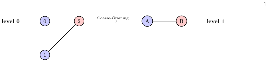
Inconsistency of the CM: a trivial example By referring to Figure 9, the microscopic network of 3 nodes 0 , 1, 2 merges into the coarse-grained network with blocks A, B, containing respectively the nodes 0 , 1 and the node 2, namely A = Ω(0) = Ω(1), B= Ω(2). Assuming having fi...
[56]

the activation function to be the same at every scale, we impose the block-parameters are the sum of their members parameters xA := (x0 + x1) and xB := x2 as for the MSM

Summed (renormalized) CM To enforce the self-consistency (scale-invariance), i.e. the activation function to be the same at every scale, we impose the block-parameters are the sum of their members parameters xA := (x0 + x1) and xB := x2 as for the MSM. With this choice, the su...
[57]

The observed network is assumed to lay at the lowest level 0, whereas the higher scales ℓ ≥ 1 identify the coarser representations obtained by aggregating the level 0 graph

Model Derivation By referring to the full derivation of the multi-scale model (MSM) [18], we report here only the crucial passages for our treatment. The observed network is assumed to lay at the lowest level 0, whereas the higher scales ℓ ≥ 1 identify the coarser representati...
[58]

For this reason, the output model is called the degree-correctedMSM (degcMSM)

Parameter Estimation In order to tackle the reconstruction problem -inferring the link probability starting from aggregated inputs-, the MSM parameters can be estimated by enforcing the degree sequence on average as done for the CM in section A. For this reason, the output mod...
[59]

However, it may happen that some nodes are deterministic, i.e

Removal of deterministic nodes Network reconstruction assumes that the observed A is a realization of a Bernoullian random process. However, it may happen that some nodes are deterministic, i.e. fully-connected (FC) or disconnected (D) to the other nodes. Therefore, their beha...
[60]

Algorithmic Complexity To describe the higher levels, one needs a lower computational complexity by means of a scale-invariant model than a single-scale (SSM) one. Specifically, the computational complexity of the RHS of Equation B8 (the only one possible to coarse-grain an SS...
[61]

The crucial point is that, even if the CM is not theoretically scale-invariant (see section A 1), it may be numerically similar to the MSM

Numerical Comparison between the CM and MSM functional form Here, we evaluated the CM and MSM functional forms for x ∈ [0, 10]. The crucial point is that, even if the CM is not theoretically scale-invariant (see section A 1), it may be numerically similar to the MSM. Actually,...
[62]

Technically, the first twos have the same functional form, while depending on the fitted and the summed parameters, respectively

Comparison Between Probabilities For every level ℓ, both CM and MSM give rise to 3 probability functions: the fitted P(ℓ) f it, summed P(ℓ) sum and the coarse-grained P(ℓ) cog. Technically, the first twos have the same functional form, while depending on the fitted and the sum...
[63]

Formally, each of such measurements is a function Y (A) of an N × N adjacency matrix representing a graph G

Degree, Average-Nearest Neighbor Degree and Clustering Coefficient The fundamental topological properties of a network are the degree, the average nearest neighbor degree (ANND) and the clustering coefficient (CC) [28]. Formally, each of such measurements is a function Y (A) o...
[64]

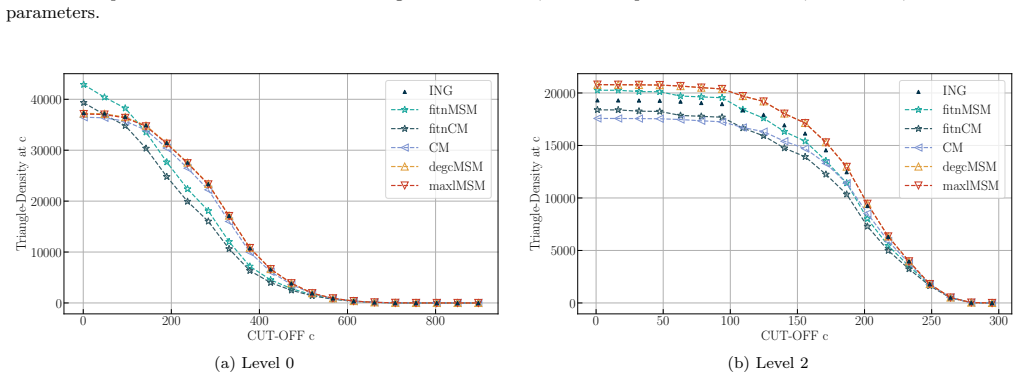
T riangle Density Inspired by [11], we computed the expected number of triangles for every model at disposal 6. Specifically, the expected density of triangles at a certain level ℓ is defined as ρ(ℓ)(c) := △(G(ℓ) kiℓ ≥c) 2Nℓ = P i̸=j̸=k gijgjk gki 2Nℓ (C13) where △(G(ℓ) kiℓ ≥c...
[65]

On the ensemble estimation For more complicated measurements, e.g. the variance of the ANND, the delta approximation won’t be valid and one has to estimate them as the average over a sufficiently large ensemble A := {As}s∈[1,S] where S is the number of graphs. In particular, h...
[66]

This measure is defined as the fraction of times an observed statistics Yi falls within the dispersion interval ∆c(⟨Yi⟩) (see section C 2)

Reconstruction Accuracy In order to have a cross-comparison among all the levels and models, we exploited the reconstruction accuracy [42]. This measure is defined as the fraction of times an observed statistics Yi falls within the dispersion interval ∆c(⟨Yi⟩) (see section C 2...
[67]

naive classifier

Rescaled ROC and PR Curves By considering the introduced models as binary classifiers it seems natural to inspect their expected confu- sion matrix, Receiver Operating Characteristic (ROC) and the Precision-Recall (PR) curves [45, 46]. In partic- ular, the expected confusion m...

Pith tools

Reviewed August 5, 2026 · model on record in the stance chip above.

[1] [1]

They require that the renormalized probability P(ℓ) sum equals the coarse-grained P(ℓ) cog with the same functional form ([18], section B 1) for all the scales

Summed MSM This class of models is defined by enforcing the follow- ing two conditions, namely    P(ℓ) sum ! = P(ℓ) cog P(ℓ) ! ≡ P(m) (19) ∀ℓ ≥ 0, m ≥ 0, which are jointly referred to as the scale-invariance (or self-consistency) properties. They require that the renormalized probability P(ℓ) sum equals the coarse-grained P(ℓ) cog with the same functio...

work page

[2] [2]

coarse-graining

Summed CM Once the microscopic ⃗ x(0) := {xi0 }i0∈[1,N0] have been estimated, the Configuration Model (CM) lacks a built-in renormalization procedure. As such, two possible strate- gies can be followed: “coarse-graining” the microscopic probabilities (Equation B6) or by refitting the parame- ters at that level ℓ. Both solutions suffer from a similar drawb...

work page

[3] [3]

Public Admin- istration

Fixed (renormalized) fitnCM Similarly to the CM, the fitnCM lacks scale-invariance properties. Therefore, we implement a renormalization scheme whereby δ(ℓ) ! = δ(0) (the latter parameter was fixed at the microscopic level 0), while the block-fitness I is obtained by summing the inner fitness {ϕi}{i∈I} (see section A). Note that this approach is equivalen...

work page 2022

[4] [4]

This does not guarantee that the predictions derived from a summed model will match those from a re-fitted one

Interlude: Scale-Invariance Implications The principle of scale-invariance, as defined in Equa- tion B5, requires that the network ensembles generated from summed and coarse-grained probabilities are sta- tistically equivalent. This does not guarantee that the predictions derived from a summed model will match those from a re-fitted one. Therefore, true d...

work page

[5] [5]

As a result, the fitnCM is expected to yield better local-level predictions compared to the MSMs (refer to 7a)

Level 0 At level 0 (see 4a), node strengths closely approximate the parameters of the Configuration Model (CM), while they tend to underestimate those of the MSMs, especially for nodes with low values. As a result, the fitnCM is expected to yield better local-level predictions compared to the MSMs (refer to 7a). As described in section III, CM and degcMSM...

work page

[6] [6]

As expected, the discrepancy in the CM is larger than that observed in the two MSMs

Level 2 4b illustrates the behavior of the summed variables xI with respect to the fitted values ˆ xI for the CM, degcMSM, and maxlMSM. As expected, the discrepancy in the CM is larger than that observed in the two MSMs. This is because the CM is a single-scale model that does not support renormalization by summing the internal weights, or by any other pr...

work page

[7] [7]

Reconstruction, Resilience and Recov- ery of Socio-Economic Networks

This level is especially peculiar, as it is the final one before the network becomes fully connected. Conse- quently, the structure is much more heterogeneous than in previous levels. Additionally, the number of nodes at this stage is the smallest among all layers, meaning that the accurate prediction of even a single node contributes more significantly t...

work page 2021

[8] [8]

C. Song, S. Havlin, and H. A. Makse, Self-similarity of complex networks, Nature 433, 392 (2005)

work page 2005