REVIEW 3 major objections 5 minor 46 references
What Can DKIST/DL-NIRSP Tell Us About Quiet-Sun Magnetism?
T0 review · 3 major / 5 minor · reviewed 2026-08-12 · deepseek-v4-flash
Pith's one-line read The paper claims that emulated DKIST/DL-NIRSP observations recover only about 71.4% and 52.6% of the ground-truth unsigned vertical Poynting flux at two photospheric heights, and that the net flux is underestimated largely because…
desk verdict Solid forward-modeling assessment of DKIST/DL-NIRSP for quiet-Sun Poynting flux, but the headline recovery fractions don't match the paper's own Table 2. read the letter →
The pith
A machine-rendered reading of the paper's core claim, the machinery that carries it, and where it could break.
The reading
What carries the argument
The machinery is a forward-model pipeline with a built-in ground truth: the MURaM magnetoconvection simulation provides the atmosphere, SIR is used twice (forward synthesis of Stokes profiles and inverse retrieval of vector fields), DL-NIRSP's point spread function and pixel scale degrade the spectra, and DAVE4VMwDV estimates the three-dimensional photospheric velocity by minimizing the residual of the ideal induction equation $\partial B_z/\partial t = -\nabla_h\cdot(B_z v_h - B_h v_z)$ together with a Doppler-velocity penalty. The vertical Poynting flux is then computed as $S_z = (1/4\pi)\int (B_h^2 v_z - (B_h\cdot v_h)B_z)\,dS$ and split into an emergence term and a shearing term. The shearing term is the key diagnostic: because it is bilinear in the horizontal magnetic field and horizontal velocity, it is the term most sensitive to azimuth-disambiguation errors and to the systematic underestimation of horizontal flows, and the paper isolates it as the main source of missing flux.
What would settle it
Rerun the same SIR plus DAVE4VMwDV pipeline on the same MURaM quiet-Sun frames after adding photon noise at the DL-NIRSP design level (e.g., $\sigma\approx 10^{-3}$ of continuum intensity) and compare the recovered unsigned and net Poynting flux fractions. If the fractions stay within a few percent of 71.4% and 52.6%, the missing flux is dominated by the underestimated horizontal velocity; if they drop substantially, the noiseless assumption is the controlling limitation.
Extended reading notes
Core claim
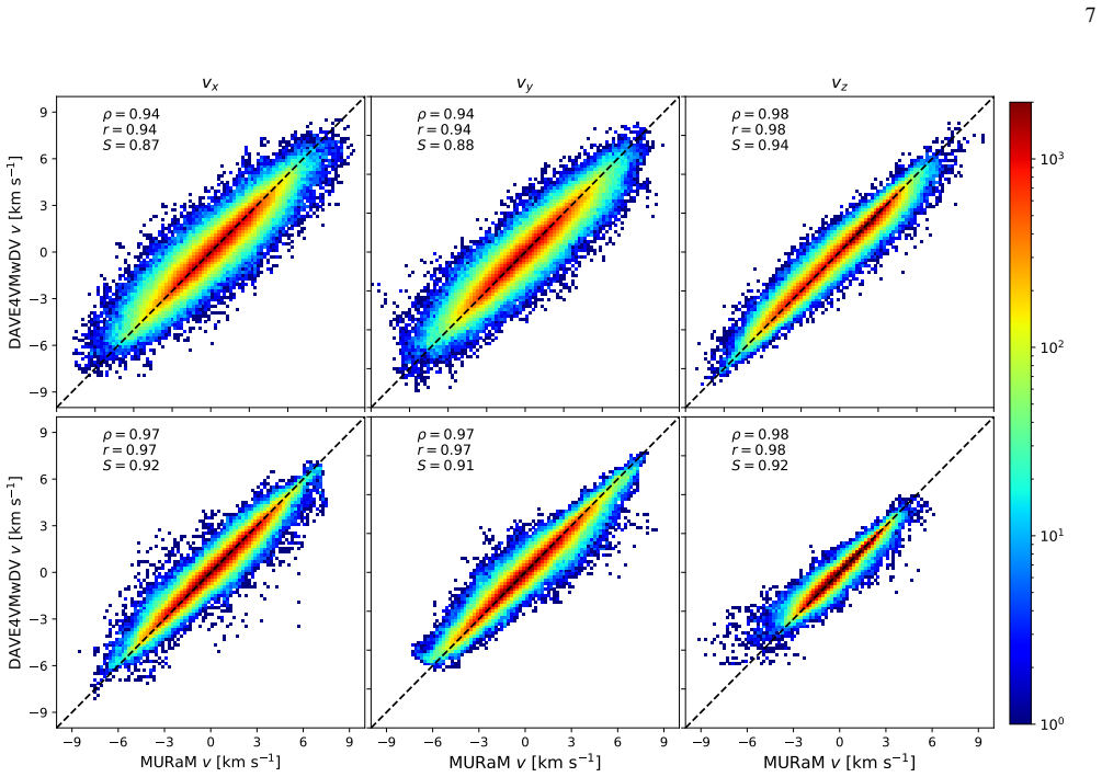
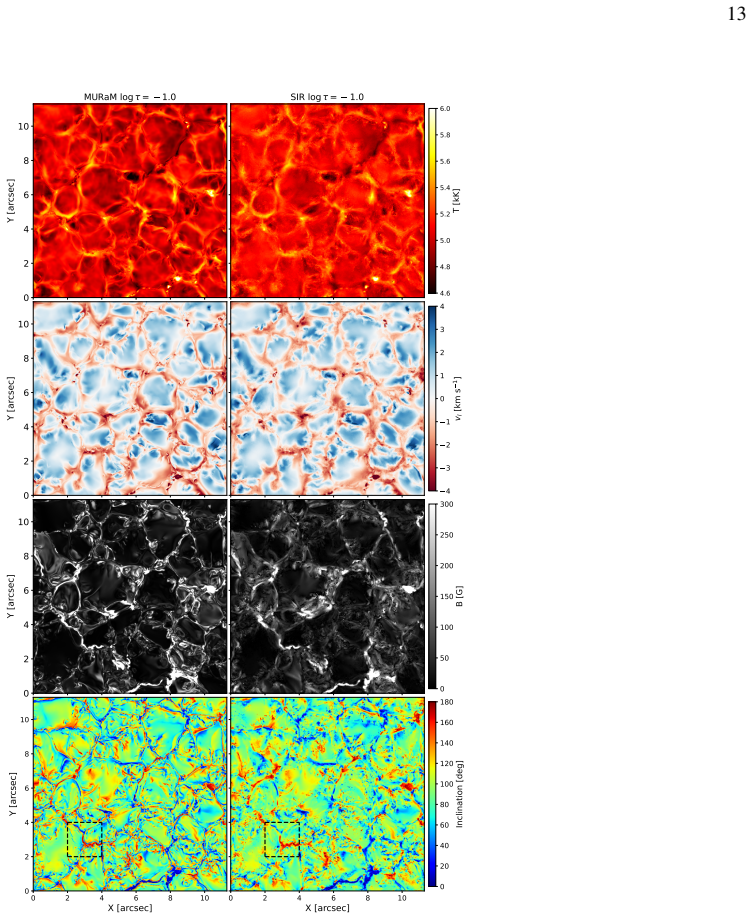
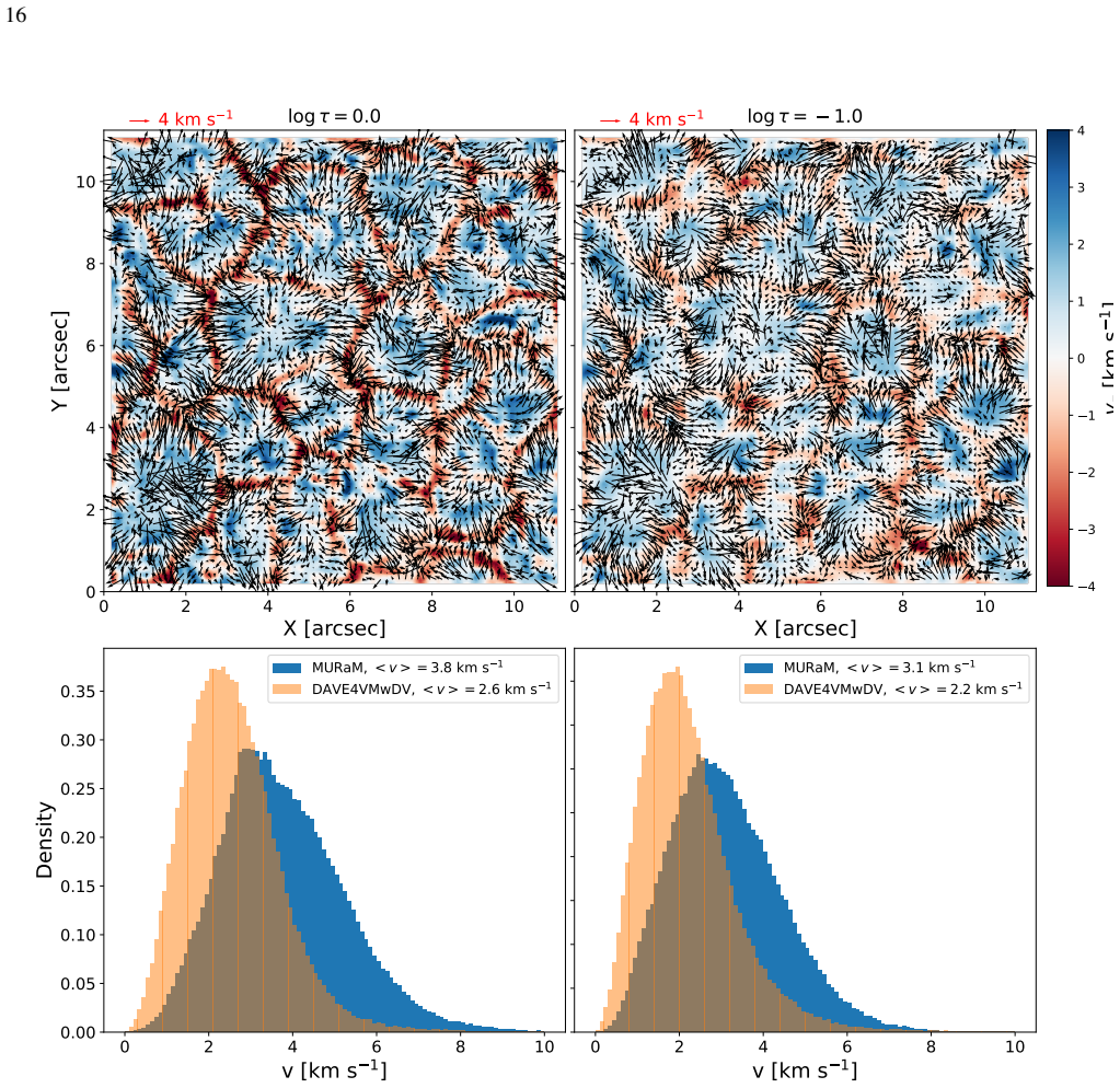
Working on a quiet-Sun magnetoconvection simulation with a mean flux density of about 120 G, the authors synthesize Stokes profiles of the Fe I 630 nm lines, convolve them with the DL-NIRSP point spread function, rebin to 0.03 arcsec pixels, and invert with SIR to obtain vector magnetic fields at constant optical depth. Velocities come from DAVE4VMwDV, a flow-tracker that fits the ideal induction equation for the vertical field while constraining the line-of-sight component to the measured Doppler velocity. The paper claims that this pipeline recovers 71.4% and 52.6% of the ground-truth unsigned vertical Poynting flux at $\log\tau=0.0$ and $\log\tau=-1.0$, but that the net vertical Poynting flux is strongly underestimated; in the emulated case at $\log\tau=0$ the inferred net flux has the wrong sign ($-1.1\times10^7$ versus $+3.7\times10^6\,\mathrm{erg\,cm^{-2}\,s^{-1}}$). Decomposition into an emergence term ($B_h^2 v_z/4\pi$) and a shearing term ($-(B_h\cdot v_h)B_z/4\pi$) shows the emergence term is recovered almost exactly on simulation magnetograms (99.6% and 88.8% of the net values), whereas the shearing term is the weak link (72.0% and 55.5%), and on the emulated data the signed shearing term drops to roughly 17% of the reference at $\log\tau=0$. The horizontal velocity field is the main culprit: DAVE4VMwDV reproduces large-scale (above roughly 150–200 km) flows well, but systematically underestimates flow amplitudes, and the shortfall worsens as cadence degrades, with an effective constraint $\Delta x/\Delta t > \langle v\rangle$ for reliable velocity estimates. The authors emphasize that photon noise was deliberately omitted, so these fractions should be read as upper limits on what the instrument chain can deliver.
Load-bearing premise
The load-bearing premise is that photon-free synthetic Stokes profiles stand in for real DL-NIRSP observations; the paper explicitly omits noise, and quiet-Sun polarization signals are weak, so actual recovery will likely be worse than the quoted fractions.
Editorial extensions
If this is right
- For DKIST/DL-NIRSP quiet-Sun campaigns, unsigned vertical Poynting flux measured with SIR plus DAVE4VMwDV should be treated as a lower limit, with the missing fraction concentrated in the shearing contribution from horizontal motions at scales below a few hundred kilometers.
- Estimates of the net vertical Poynting flux, and any conclusion about net upward versus downward magnetic energy transport, are not reliable with current schemes: the sign itself can be wrong at photospheric heights.
- Velocity products from DAVE4VMwDV are trustworthy only at scales larger than roughly 150–200 km; users should not interpret small-scale flow structure recovered by the algorithm as real.
- Cadence planning matters: to keep velocity estimates accurate, magnetogram cadence should satisfy $\Delta x/\Delta t > \langle v\rangle$, corresponding to roughly 2.5 s or better for 16 km pixels, which DL-NIRSP's several-second cadence can approach but may not always reach.
- Improvements that place inversions on constant geometric height, such as magnetohydrostatic inversions or deep-learning methods, can recover an additional 10–20 percentage points of the shearing term, so the missing flux is a recoverable systematic rather than an intrinsic ceiling.
Reading between the lines
- Inference: because the pipeline is noiseless, the 71.4% and 52.6% recovery fractions are optimistic ceilings; real DL-NIRSP data with photon noise on weak quiet-Sun polarization will likely recover a smaller fraction, and the net flux sign may be even less trustworthy.
- Inference: the paper's scale analysis implies that a correction function could be calibrated from simulation—recovery fraction as a function of pixel size, cadence, and noise level—and applied to real DL-NIRSP observations in future quiet-Sun energy-budget studies.
- Inference: the specific failure mode, azimuth ambiguity corrupting $v_h\cdot B_h$, suggests that multi-height or multi-line inversions that resolve the 180-degree ambiguity without a smoothness prior would be the single highest-leverage upgrade over the current scheme.
- Inference: the result generalizes beyond DKIST: any spectropolarimetric quiet-Sun Poynting-flux measurement using similar flow-tracking will be biased low, so comparisons between instruments such as Hinode, SUNRISE, and DKIST should be made on recovery-corrected quantities rather than raw fluxes.
Editorial analysis
A structured set of objections, weighed in public.
Referee Report
Summary. This paper assesses the diagnostic capability of DKIST/DL-NIRSP for quiet-Sun magnetism by constructing an end-to-end pipeline: synthetic Stokes profiles from a MURaM simulation are degraded to emulate DL-NIRSP observations, inverted with SIR to obtain vector magnetic fields, processed with the DAVE4VMwDV algorithm to estimate photospheric velocities, and then used to compute vertical Poynting flux. The authors validate the velocity inference on high-resolution simulation data, investigate dependence on cadence, and evaluate the recovery of Poynting flux from the emulated observations. The central quantitative claim is that the unsigned Poynting flux can be recovered at about 71.4% (log τ=0.0) and 52.6% (log τ=-1.0) of the ground truth, with the net flux strongly underestimated and the shearing term identified as the main source of error. The paper also provides scale-based guidance for required velocity resolution and discusses limitations due to the constant-τ surface, azimuthal disambiguation, and the absence of photon noise.
Significance. If the quantitative results were internally consistent, this would be a valuable end-to-end assessment of what DKIST/DL-NIRSP can deliver for quiet-Sun energy transport studies. The pipeline uses an independent MHD simulation as ground truth, explicitly analyzes the limitations of constant-τ magnetograms for flow tracking, and offers concrete guidance on required spatial and temporal scales for recovering the emergence and shearing terms of the Poynting flux. The paper is also transparent about many known limitations, such as the noiseless assumption and the poor performance of the ME0 disambiguation. However, the central recovery percentages are mutually inconsistent across the abstract, main text, and conclusion, and they do not follow from Table 2. Until these numbers are reconciled, the paper's headline quantitative conclusion is not reproducible from the presented evidence.
major comments (3)
- [Abstract, Section 4.2, Section 6, Table 2] The net Poynting flux values quoted in the conclusion differ from Table 2: the conclusion lists -1.3×10^7 and -8.5×10^6 erg cm^-2 s^-1, while Table 2 gives -10.5×10^6 and -8.6×10^6. This is another instance of the same numerical inconsistency.
- [Section 2.2, Section 5.4] The noiseless emulation is an acknowledged but understated limitation. Section 2.2 states 'We did not add noise to the synthetic spectra for this study,' and Section 5.4 defers noise effects to future work. For quiet-Sun Stokes Q, U, and V signals, photon noise is expected to be a dominant error source, so the quoted recovery percentages are optimistic upper limits rather than realistic capability estimates. The abstract and conclusion present these numbers without this caveat. The authors should either add a noise sensitivity analysis (e.g., a single representative noise level) or explicitly qualify the headline numbers as noiseless, idealized recoveries.
- [Appendix A.2] The DAVE4VMwDV free parameters (λ, d, dr, w) are optimized on the same emulated observation data that are then used to evaluate the Poynting flux recovery. This in-sample tuning means the reported recovery fractions are not out-of-sample estimates; the L-curve and L1-minimization procedures in Appendix A select parameters that best fit the specific realization. The paper should demonstrate robustness to parameter choices, for example by showing the range of recovery fractions across a plausible parameter grid or by fixing the parameters a priori based on the simulation-data experiments in Appendix A.1.
minor comments (5)
- [Equation (9)] The definition of E_rel appears malformed: the numerator should be the Euclidean norm of the difference vector and the denominator should be the product of the vector magnitudes, not the dot product as written. As printed, the denominator can be zero or negative, making the metric ill-defined.
- [Section 1] In the first paragraph, 'Goiet al. 2014, 2016' is missing a space; it should read 'Goi et al. 2014, 2016'.
- [Section 4.2] The text states 'The inferred unsigned Poynting flux is 2.0 × 10^8 ergs cm^-2 s^-1', but Table 2 gives 150.5 × 10^6 = 1.505 × 10^8 erg cm^-2 s^-1. The value 2.0 × 10^8 is inconsistent by about 33%.
- [Section 4.2] The percentage for the unsigned shearing term is quoted as 44.6% of the ground truth, while Table 2 implies 95.2/201.1 = 47.3%. Please check the calculation.
- [Section 3.1 and Figure 4 caption] The phrase 'Here and after' should be 'Hereafter' for clarity.
Circularity Check
No constructional circularity: recovery fractions are benchmarked against independent MURaM truth; the only circularity-adjacent burden is a co-author's in-preparation flow-tracking code with in-sample parameter tuning, plus a separate internal numerical inconsistency in the headline percentages.
-
other
[Section 2.4 (Eq. 6) and Appendix A]
"Termed DA VE4VMwDV (with Doppler Velocity; P. W. Schuck 2024, in preparation), the global loss function L now reads ... In this work, we optimize these parameters using the methods described in Liu et al. (2023)."
The flow-tracking step that supplies the velocities for every downstream Poynting-flux number is an unpublished algorithm attributed to a co-author, and its free parameters are selected by minimizing the loss on the same emulated data used for the capability assessment. This makes the reported recovery fractions in-sample and potentially optimistic, and it places a self-citation burden on the method's provenance. It is not a full constructional circularity because the comparison ground truth comes from the independent MURaM simulation, so the recovery fractions are not equated to a fitted input by definition.
full rationale
The derivation chain is self-contained against an external benchmark. MURaM provides ground-truth B and v; SIR synthesizes and inverts the Stokes profiles; DAVE4VMwDV estimates the velocity from the magnetogram/Dopplergram sequence; Equation (8) computes the Poynting flux; and every estimate is compared with the simulation truth. The induction equation is used as a physical constraint rather than as a fit to the Poynting-flux target, so the central result does not reduce to its inputs by construction. The noiseless-emulation caveat is explicitly stated in Section 2.2 ('We did not add noise to the synthetic spectra for this study'), making the numbers optimistic limits rather than full capability bounds; this is a limitation, not a circular step. The minor circularity-adjacent concern is the in-preparation, co-authored DAVE4VMwDV and in-sample hyperparameter selection, which is why the score is not 0. Separately, the paper has an internal numerical inconsistency: the abstract's 71.4%/52.6% unsigned-Poynting recovery fractions do not match Table 2's emulation rows (150.5/278.9 = 53.9% and 36.2/75.7 = 47.8%), while the conclusion reports 72.5%/61.3%; this is a reproducibility/correctness defect that should be fixed but is not itself circularity.
Assumptions & free parameters
free parameters (5)
- DAVE4VMwDV window size w =
15 pixels for all runs
- DAVE4VMwDV Legendre degrees (d, dr) =
(5,7) at log tau=0 and (3,5) at log tau=-1 for MHD data; (3,5) and (1,5) for emulated data
- DAVE4VMwDV Doppler weighting lambda =
1.0 for MHD data, 0.35 for emulated data
- ME0 disambiguation weighting lambda =
0.5
- SIR node configuration =
Table 1: 5 nodes for magnetic field, inclination, azimuth in final cycles; experiment two uses 14, 14, 5
assumptions (5)
- domain assumption MURaM O16bM simulation is a realistic representation of quiet-Sun magnetoconvection
- domain assumption SIR inversion under LTE and hydrostatic equilibrium recovers depth-dependent atmospheric parameters
- domain assumption The ideal induction equation holds on constant-tau surfaces for velocity inference
- domain assumption ME0 minimum-energy disambiguation selects correct azimuths in the quiet Sun
- ad hoc to paper Noise-free synthetic Stokes profiles are sufficient to assess DL-NIRSP diagnostic capability
Cite this review
Pith. "Pith review of What Can DKIST/DL-NIRSP Tell Us About Quiet-Sun Magnetism?." pith.science (2026). https://pith.science/paper/DH54MOOC
@misc{pith2026241118735,
  author       = {Pith},
  title        = {Pith review of: What Can DKIST/DL-NIRSP Tell Us About Quiet-Sun Magnetism?},
  year         = {2026},
  howpublished = {\url{https://pith.science/paper/DH54MOOC}},
  note         = {Machine review of arXiv:2411.18735}
}
abstract
Quiet-Sun regions cover most of the Sun's surface; its magnetic fields contribute significantly to the solar chromospheric and coronal heating. However, characterizing the magnetic fields of the quiet Sun is challenging due to their weak polarization signal. The 4-m \textit{Daniel K. Inouye Solar Telescope} (\textit{DKIST}) is expected to improve our understanding of the quiet-Sun magnetism. In this paper, we assess the diagnostic capability of the Diffraction-Limited Near Infrared Spectropolarimeter (DL-NIRSP) instrument on \textit{DKIST} on the energy transport processes in the quiet-Sun photosphere. To this end, we synthesize high-resolution, high-cadence Stokes profiles of the \ion{Fe}{1} 630~nm lines using a realistic magnetohydrodynamic simulation, degrade them to emulate the \textit{DKIST}/DL-NIRSP observations, and subsequently infer the vector magnetic and velocity fields. For the assessment, we first verify that a widely used flow-tracking algorithm, Differential Affine Velocity Estimator for Vector Magnetograms, works well for estimating the large-scale ($> 200$ km) photospheric velocity fields with these high-resolution data. We then examine how the accuracy of inferred velocity depends on the temporal resolution. Finally, we investigate the reliability of the Poynting flux estimate and its dependence on the model assumptions. The results suggest that the unsigned Poynting flux, estimated with existing schemes, can account for about $71.4\%$ and $52.6\%$ of the reference ground truth at $\log \tau =0.0$ and $\log \tau = -1$. However, the net Poynting flux tends to be significantly underestimated. The error mainly arises from the underestimated contribution of the horizontal motion. We discuss the implications on \textit{DKIST} observations.
Figures


Figures from the paper (19 more)






Reference graph
Works this paper leans on
-
[1]
, " * write output.state after.block = add.period write newline
ENTRY address archivePrefix author booktitle chapter doi edition editor eprint howpublished institution journal key month number organization pages publisher school series title misctitle type volume year version url label extra.label sort.label short.list INTEGERS output.state before.all mid.sentence after.sentence after.block FUNCTION init.state.consts ...
-
[2]
write newline
" write newline "" before.all 'output.state := FUNCTION format.url url empty "" new.block "" url * "" * if FUNCTION format.eprint eprint empty "" archivePrefix empty "" archivePrefix "arXiv" = new.block " " eprint * " " * new.block " " eprint * " " * if if if FUNCTION format.doi doi empty "" " " doi * " " * if FUNCTION format.pid doi empty eprint empty ur...
-
[3]
thebibliography [1] 20pt to REFERENCES 6pt =0pt -12pt 10pt plus 3pt =0pt =0pt =1pt plus 1pt =0pt =0pt -12pt =13pt plus 1pt =20pt =13pt plus 1pt \@M =10000 =-1.0em =0pt =0pt 0pt =0pt =1.0em @enumiv\@empty 10000 10000 `\.\@m \@noitemerr \@latex@warning Empty `thebibliography' environment \@ifnextchar \@reference \@latexerr Missing key on reference command E...
-
[4]
Alissandrakis , C. E., & Gary , D. E. 2021, Frontiers in Astronomy and Space Sciences, 7, 77, 10.3389/fspas.2020.591075
arXiv 2021
-
[5]
Asensio Ramos , A., & D \' az Baso , C. J. 2019, , 626, A102, 10.1051/0004-6361/201935628
-
[6]
Asensio Ramos , A., Requerey , I. S., & Vitas , N. 2017, , 604, A11, 10.1051/0004-6361/201730783
-
[7]
2019, Living Reviews in Solar Physics, 16, 1, 10.1007/s41116-018-0017-1
Bellot Rubio , L., & Orozco Su \'a rez , D. 2019, Living Reviews in Solar Physics, 16, 1, 10.1007/s41116-018-0017-1
-
[8]
Berghmans , D., Auch \`e re , F., Long , D. M., et al. 2021, , 656, L4, 10.1051/0004-6361/202140380
Show all 46 references
-
[9]
Danilovic , S., Sch \"u ssler , M., & Solanki , S. K. 2010, , 513, A1, 10.1051/0004-6361/200913379
2010 doi
-
[10]
G., Lites, B
de Wijn, A. G., Lites, B. W., Berger, T. E., et al. 2008, The Astrophysical Journal, 684, 1469, 10.1086/590237
2008 doi
-
[11]
C., & Ruiz Cobo , B
del Toro Iniesta , J. C., & Ruiz Cobo , B. 2016, Living Reviews in Solar Physics, 13, 4, 10.1007/s41116-016-0005-2
2016 doi
-
[12]
J., Brun , A
Finley , A. J., Brun , A. S., Carlsson , M., et al. 2022, , 665, A118, 10.1051/0004-6361/202243947
2022 doi
-
[13]
M., Avrett , E., Thuillier , G., & Harder , J
Fontenla , J. M., Avrett , E., Thuillier , G., & Harder , J. 2006, , 639, 441, 10.1086/499345
2006 doi
-
[14]
2020, , 904, 7, 10.3847/1538-4357/abbb36
Giannattasio , F., Consolini , G., Berrilli , F., & Del Moro , D. 2020, , 904, 7, 10.3847/1538-4357/abbb36
2020 doi
-
[15]
Gošić, M., Rubio, L. R. B., del Toro Iniesta, J. C., Suárez, D. O., & Katsukawa, Y. 2016, The Astrophysical Journal, 820, 35, 10.3847/0004-637X/820/1/35
2016 doi
-
[16]
Gošić, M., Rubio, L. R. B., Suárez, D. O., Katsukawa, Y., & del Toro Iniesta, J. C. 2014, The Astrophysical Journal, 797, 49, 10.1088/0004-637X/797/1/49
2014 doi
-
[17]
Hale , G. E. 1908, , 28, 315, 10.1086/141602
1908 doi
-
[18]
C., & O'Leary, D
Hansen, P. C., & O'Leary, D. P. 1993, SIAM Journal on Scientific Computing, 14, 1487, 10.1137/0914086
1993 doi
-
[19]
A., Lin , H., Onaka , P., et al
Jaeggli , S. A., Lin , H., Onaka , P., et al. 2022, , 297, 137, 10.1007/s11207-022-02062-w
2022 doi
-
[20]
B., Jafarzadeh , S., Keys , P
Jess , D. B., Jafarzadeh , S., Keys , P. H., et al. 2023, Living Reviews in Solar Physics, 20, 1, 10.1007/s41116-022-00035-6
2023 doi
-
[21]
2002, , 577, 501, 10.1086/342171
Kusano , K., Maeshiro , T., Yokoyama , T., & Sakurai , T. 2002, , 577, 501, 10.1086/342171
2002 doi
-
[22]
D., Barnes , G., Crouch , A
Leka , K. D., Barnes , G., Crouch , A. D., et al. 2009, , 260, 83, 10.1007/s11207-009-9440-8
2009 doi
-
[23]
W., et al
Liu , J., Sun , X., Schuck , P. W., et al. 2023, , 955, 40, 10.3847/1538-4357/ace907
2023 doi
-
[24]
Longcope , D. W. 2004, , 612, 1181, 10.1086/422579
2004 doi
-
[25]
Metcalf , T. R. 1994, , 155, 235, 10.1007/BF00680593
1994 doi
-
[26]
R., Leka , K
Metcalf , T. R., Leka , K. D., Barnes , G., et al. 2006, , 237, 267, 10.1007/s11207-006-0170-x
2006 doi
- [27]
-
[28]
1991, , 135, 179, 10.1007/BF00146705
Moran , T., & Foukal , P. 1991, , 135, 179, 10.1007/BF00146705
1991 doi
-
[29]
, Bellot Rubio, L
Orozco Su\'arez, D. , Bellot Rubio, L. R. , Mart\' nez Pillet, V. , et al. 2010, A&A, 522, A101, 10.1051/0004-6361/201014217
2010 doi
-
[30]
M., & Ruiz Cobo , B
Pastor Yabar , A., Borrero , J. M., & Ruiz Cobo , B. 2019, , 629, A24, 10.1051/0004-6361/201935692
2019 doi
-
[31]
2023, , 675, A93, 10.1051/0004-6361/202345890
Quintero Noda , C., Khomenko , E., Collados , M., et al. 2023, , 675, A93, 10.1051/0004-6361/202345890
2023 doi
-
[32]
P., Bello Gonz \'a lez , N., Bellot Rubio , L., et al
Rast , M. P., Bello Gonz \'a lez , N., Bellot Rubio , L., et al. 2021, , 296, 70, 10.1007/s11207-021-01789-2
2021 doi
-
[33]
2014, The Astrophysical Journal, 789, 132, 10.1088/0004-637X/789/2/132
Rempel, M. 2014, The Astrophysical Journal, 789, 132, 10.1088/0004-637X/789/2/132
2014 doi
-
[34]
R., Warner , M., Keil , S
Rimmele , T. R., Warner , M., Keil , S. L., et al. 2020, , 295, 172, 10.1007/s11207-020-01736-7
2020 doi
-
[35]
Ruiz Cobo , B., & del Toro Iniesta , J. C. 1992, , 398, 375, 10.1086/171862
1992 doi
-
[36]
J., De Rosa , M
Schrijver , C. J., De Rosa , M. L., Metcalf , T. R., et al. 2006, , 235, 161, 10.1007/s11207-006-0068-7
2006 doi
-
[37]
Schuck , P. W. 2006, , 646, 1358, 10.1086/505015
2006 doi
- [38]
-
[39]
2023, , 956, 83, 10.3847/1538-4357/ace621
Tilipman , D., Kazachenko , M., Tremblay , B., et al. 2023, , 956, 83, 10.3847/1538-4357/ace621
2023 doi
-
[40]
2020, Frontiers in Astronomy and Space Sciences, 7, 25, 10.3389/fspas.2020.00025
Tremblay , B., & Attie , R. 2020, Frontiers in Astronomy and Space Sciences, 7, 25, 10.3389/fspas.2020.00025
2020
-
[41]
2012, A&A, 548, A5, 10.1051/0004-6361/201220220
van Noort, M. 2012, A&A, 548, A5, 10.1051/0004-6361/201220220
2012 doi
-
[42]
o gler , A., Shelyag , S., Sch \
V \"o gler , A., Shelyag , S., Sch \"u ssler , M., et al. 2005, , 429, 335, 10.1051/0004-6361:20041507
2005 doi
-
[43]
T., Fisher , G
Welsch , B. T., Fisher , G. H., Abbett , W. P., & Regnier , S. 2004, , 610, 1148, 10.1086/421767
2004 doi
-
[44]
T., Abbett , W
Welsch , B. T., Abbett , W. P., De Rosa , M. L., et al. 2007, , 670, 1434, 10.1086/522422
2007 doi
-
[45]
E., Tarr , L
Yang , K. E., Tarr , L. A., Rempel , M., et al. 2024, arXiv e-prints, arXiv:2407.20309, 10.48550/arXiv.2407.20309
2024 doi
-
[46]
P., Wang , J
Zhou , G. P., Wang , J. X., & Jin , C. L. 2010, , 267, 63, 10.1007/s11207-010-9641-1
2010 doi
Reviewed August 12, 2026 · model on record in the stance chip above.
Discussion (0). Continue with ORCID to comment.