REVIEW 4 major objections 5 minor 14 references
Leveraging NMF to Investigate Air Quality in Central Taiwan
T0 review · 4 major / 5 minor · reviewed 2026-08-12 · deepseek-v4-flash
Pith's one-line read Factoring a decade of hourly readings from 14 stations, the paper concludes that NO2 and PM2.5 in central Taiwan are mostly local, SO2 mostly imported, and PM10 split nearly evenly.
desk verdict Table 3 is internally inconsistent and unvalidated; the paper's central claim is not supported by its own analysis. read the letter →
The pith
A machine-rendered reading of the paper's core claim, the machinery that carries it, and where it could break.
The reading
What carries the argument
The load-bearing object is the NMF factorization $A \approx WH$, with $W$ the time profiles and $H$ the spatial loadings of $k$ source components, computed by multiplicative update rules that keep every entry non-negative; non-negativity is what lets each component be read as an additive, physically meaningful source profile. Around it sits the cophenetic-correlation rule for choosing $k$ and, decisively, the wind-rose inspection that assigns each component to 'domestic' or 'transboundary' by the wind speed at which its pollution load concentrates. The wind-speed signature is what converts a statistical factorization into a geographic attribution.
What would settle it
Recompute the source-apportionment table with a single explicit wind-speed cutoff — for example the 5.5 m/s boundary of the paper's own wind classification, or 6 m/s — applied uniformly to every NMF component, and rerun the validation using the same component counts as the main analysis: if NO2's domestic share falls below half, or if the validation procedure does not reproduce the main proportions when applied to the full 2008–2017 record, the central claim fails.
Extended reading notes
Core claim
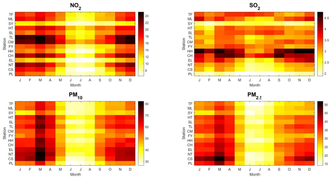
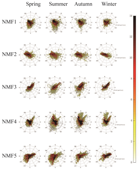
The discovery, stated on the paper's own terms, is a source-apportionment table: over 2008–2017 in central Taiwan, NO2 is 66.36% domestic and 33.64% transboundary, PM2.5 is 64.65% domestic, SO2 is 45.83% domestic (54.17% transboundary), and PM10 is 50.95% domestic (49.05% transboundary). These numbers come from decomposing each pollutant's $87{,}672 \times 14$ hourly matrix into spatial and temporal factors with non-negative matrix factorization, choosing the number of factors by cophenetic correlation, and then reading each factor's wind rose: factors whose pollution concentrates at gentle wind speeds around 3.5–4.8 m/s are classified as domestic, while factors driven by monsoon winds of 7–12 m/s are classified as transboundary. The paper further claims that this classification scheme is validated by comparing a 2010 re-run of the procedure, with larger numbers of factors, against an independently estimated 2010 domestic-ratio benchmark, finding agreement within about six percentage points for NO2, SO2, and O3.
Load-bearing premise
The load-bearing premise is that a pollutant component's wind speed alone, read visually from a wind rose, cleanly separates 'domestic' from 'transboundary' sources: components peaking near 4 m/s are called domestic and those reaching roughly 7 to 12 m/s are called transboundary, with no quantitative threshold, error margin, or physical transport model behind the split; changing that cutoff directly changes every percentage in the results table.
Editorial extensions
If this is right
- For NO2 and PM2.5, the policy lever is local: vehicle, industrial, and power-plant controls inside central Taiwan would address the domestic majority of these pollutants.
- For SO2, local abatement alone would leave more than half the burden in place, so reducing SO2 requires cooperation with sources across the Taiwan Strait.
- For PM10, domestic and transboundary measures carry roughly equal weight, so neither a purely local nor a purely regional strategy is sufficient.
- The SO2 peaks recorded at the station downwind of the Taichung thermal power plant are attributed to transboundary flow, implying the plant's local SO2 fingerprint is, by this method, small relative to imported SO2.
- If the method is right, the 2010 benchmark agreement (within about six percentage points for NO2, SO2, and O3) indicates the same pipeline can be reused for other pollutants and other years without redesigning the analysis.
Reading between the lines
- A direct test the paper leaves unwritten: refit the classification with one explicit wind-speed cutoff (for instance the 5.5 m/s 'gentle breeze' boundary of its own wind classification) applied uniformly, and watch whether NO2 and PM2.5 stay majority domestic; the percentages in the table move with the cutoff.
- The validation section examines 2010 only and uses different numbers of components than the main runs; comparing each separate year of the decade, or re-running the 2010 validation at the main component counts, would show whether the domestic-majority claim is stable or an artifact of the chosen factor count.
- Plugging the same factors into back-trajectory or chemical-transport modeling would let each NMF component be named by its actual airmass origin, turning the visual wind-speed heuristic into a falsifiable source attribution.
- If the domestic/transboundary proportions survive such tests, they give both Taiwan's local governments and cross-strait negotiators a concrete basis for allocating abatement costs.
Editorial analysis
A structured set of objections, weighed in public.
Referee Report
Summary. The paper applies non-negative matrix factorization (NMF) to hourly air-quality data for SO2, NO2, PM10, and PM2.5 from 14 monitoring stations in central Taiwan over 2008–2017 (87,672 hourly records). For each pollutant the data matrix is decomposed into k components; each component is then classified as 'domestic' or 'transboundary' based on wind-rose patterns, and the component shares are aggregated into Table 3, which reports domestic/transboundary proportions of 66.36%/33.64% for NO2, 45.83%/54.17% for SO2, 50.95%/49.05% for PM10, and 64.65%/35.35% for PM2.5. The paper concludes that NO2 and PM2.5 are domestically dominated, SO2 is substantially transboundary, and PM10 is nearly balanced. Section 6 re-runs the analysis on 2010 data with different k values (k=8 for NO2, k=10 for O3 and SO2) and compares the resulting domestic ratios against Chen et al. (2010), reporting agreement within a claimed ±6% margin.
Significance. If the reported proportions were robust, the paper would provide useful quantitative input for central Taiwan's air-quality policy, separating domestic from transboundary contributions. The study has several strengths: NMF is a reasonable tool for nonnegative compositional data; the validation against independent 2010 estimates from Chen et al. is a good idea; and including O3 as a sanity check (even though O3 is not part of the headline results) shows an attempt at external grounding. However, the paper ships no code, no data-availability statement, no error bars, and no sensitivity analysis for the classification rule. More importantly, the headline percentages in Table 3 are not backed by the manuscript's own component classifications, and the validation in Section 6 uses a re-configured version of the method rather than the main analysis. If the internal inconsistency and validation gap were fixed, the qualitative finding—especially for SO2 and PM10—could still be defensible, but the quantitative claims in Table 3 are not currently supported.
major comments (4)
- [Section 5, Table 3] The NO2 row of Table 3 is internally inconsistent with the component classifications given in Section 5. The text labels NMF1, NMF2, and NMF4 as domestic (16.79%, 16.58%, 16.43%) and NMF3, NMF5, and NMF6 as transboundary (16.58%, 16.68%, 16.56%). Summing the domestic shares gives 49.80%, not 66.36%; the table's 66.36% is recovered only by counting NMF6—explicitly called transboundary in the text—as domestic. This is a load-bearing arithmetic error because the abstract's statement that NO2 is 'primarily influenced by local sources' hinges on this row.
- [Section 6 vs Table 3] The validation in Section 6 does not actually validate Table 3. The main analysis uses k=6 for NO2, k=5 for SO2, k=4 for PM10, and k=3 for PM2.5 on the full 2008–2017 record, while Section 6 uses k=8 for NO2 and k=10 for O3 and SO2 on 2010 data only. For SO2, Table 3 reports 45.83% domestic for 2008–2017, but the 2010 k=10 run yields 26.92% domestic—an 18.9-percentage-point difference that is far outside the '±6% margin' claimed in Section 7. The paper never discusses this discrepancy; the conclusion's claim that the method is effective is therefore not supported for the headline results.
- [Section 5, classification rule] The domestic/transboundary attribution is made by a visual inspection of wind roses without any quantitative decision rule or sensitivity analysis. For example, in the NO2 analysis, NMF1 is called domestic because high pollution is concentrated at 4 m/s, and NMF2 is domestic at 3.5 m/s, but NMF6—with high pollution concentrated at 3.9 m/s—is classified as transboundary with no stated meteorological justification. Changing the implicit threshold by a few m/s would directly alter every percentage in Table 3. A sensitivity analysis, an objective classifier based on wind direction and speed distributions, or at least a clear statement of the applied rule with error margins is needed.
- [Section 4.1 and Section 5] The k-selection text is ambiguous and inconsistent with the displayed numbers of components. Section 4.1 describes Figures 5(a)–(d) as 'k=6 and k=5' and 'k=4 and k=3' without stating which pollutant each panel refers to, and the text does not clearly explain which k is chosen for each pollutant. The Results section then uses six components for NO2 (although Figure 6's caption says 'five components'), five for SO2, four for PM10, and three for PM2.5. The link between the cophenetic-correlation panels and the chosen k must be stated explicitly, and the figure captions should match the number of components actually used.
minor comments (5)
- [Section 1] The roadmap in the introduction says 'Section 2 outlines the methods, Section 3 describes data sources, Section 4 presents the analysis results, followed by a validation of the proposed method in Section 5. Section 6 concludes the study,' but the actual structure is Section 4 (analysis), Section 5 (results), Section 6 (validation), Section 7 (conclusion). Please correct the roadmap.
- [Table 2] The seasonal percentages for SO2 in Table 2 sum to 99.99% rather than 100%; check the rounding and report consistent totals.
- [Figures 13 and 16] The PM2.5 analysis in Section 5 refers to 'Fig. 13 reveals distinct seasonal variations,' but Figure 13 is the PM10 day-to-year variation plot. The PM2.5 day-to-year variation is shown in Figure 16.
- [Section 2, Eq. (4)–(6)] In the derivation of the multiplicative update rules, the notation '(W H H^T)' should be written as '((W H) H^T)' to avoid ambiguity about the order of multiplication; this is a presentation issue only.
- [References] Reference [14] is cited as 'Chen et al.' but the entry lists the journal as 'Science of the Total Environment, Atmospheric Environment'—two journal names—and should be corrected; also consider adding a data-availability or code-availability statement, since the public EPA data link is given but the analysis code is not.
Circularity Check
The 2010 validation is fitted by choosing k after seeing the benchmark, and the domestic/transboundary labels are built into the wind-speed heuristic, so Table 3 and Table 4 do not independently support the headline source attribution.
-
fitted input called prediction
[Section 6, 'Analysis on SO2' and Table 4]
"We have chosen not to select k = 3 or k = 5 in order to preserve the integrity of the data, opting instead for k = 10, as illustrated in Fig. 26. ... In conclusion, for the year 2010, domestic SO2 pollution represented 26.92%, while transboundary pollution accounted for 73.08%."
The external benchmark being validated is Chen et al.'s 27% domestic SO2. The main analysis used k=5 and reported 45.83% domestic (Table 3), but the validation explicitly rejects k=5 and adopts k=10, which yields 26.92% domestic, essentially the benchmark value. Because k fixes the NMF decomposition and therefore which components are subsequently labeled domestic or transboundary, selecting k after seeing the target makes the Table 4 agreement a fitted result rather than an independent confirmation. The validation does not test the k=5 headline SO2 figure.
-
renaming known result
[Section 5 (Results) and Table 3]
"NMF1 is notably influenced by westerly winds, with high pollution levels concentrated at a wind speed of 4 m/s, as shown in Fig. 8. Based on this, we classify NMF1 as domestic pollution, contributing 16.79% of all features. ... NMF3 ... wind speeds reaching up to 12 m/s ... classify NMF3 as transboundary pollution, accounting for 16.58% of all features."
The source categories are operationalized by a wind-speed rule: components peaking near 4 m/s are called domestic, while components reaching 7-12 m/s are called transboundary. Table 3 is then simply the sum of the shares of components carrying these labels. The conclusion that NO2 and PM2.5 are predominantly domestic while SO2 is transboundary is therefore a restatement of the low-versus-high wind-speed pattern imposed on the NMF components, not an independently measured source attribution. The external Chen et al. anchor is applied in Section 6 to a different k configuration, so it does not independently calibrate the Section 5 labels.
full rationale
The paper's NMF mathematics is standard and not circular, and no load-bearing self-citation chain is present. The circularity lies in the validation and labeling chain. In Section 6, the validation runs use different k values than the main analysis (NO2 k=8 instead of 6, SO2 k=10 instead of 5) and, for SO2, the authors state they deliberately avoided k=3 and k=5 before choosing k=10, which produces a domestic ratio almost identical to Chen et al.'s 27%. This is a fitted parameter choice presented as independent validation. Additionally, the main Table 3 percentages are the direct arithmetic of the Section 5 wind-speed classification rule, so the headline finding is a renaming of the wind-speed pattern rather than a source-attribution result calibrated by an external check. There is also a non-circular correctness problem: the NO2 row of Table 3 (66.36% domestic) cannot be reproduced from the Section 5 labels, where NMF1, NMF2, and NMF4 are domestic and NMF3, NMF5, and NMF6 are transboundary, which sums to 49.8% domestic; the printed figure is recovered only by counting the transboundary-labeled NMF6 as domestic. This inconsistency does not itself make the argument circular, but it further means Table 3 is not a reliable output of the stated derivation chain. Overall, the validation step reduces to post-hoc parameter selection and the headline attribution reduces to the labeling heuristic, so the circularity score is moderate-to-high.
Assumptions & free parameters
free parameters (3)
- number of components k =
5 (NO2), 5 (SO2), 4 (PM10), 3 (PM2.5) in main analysis; 8, 10, 10 in validation
- wind speed classification thresholds =
not specified numerically; examples include 4 m/s for domestic and 12 m/s for transboundary
- component labeling (domestic vs transboundary) =
manual assignment per component
assumptions (3)
- domain assumption Each NMF component corresponds to a single pollution source regime (domestic or transboundary)
- domain assumption Wind speed is a sufficient proxy for transport distance
- standard math NMF with non-negative data gives meaningful, stable factors
Cite this review
Pith. "Pith review of Leveraging NMF to Investigate Air Quality in Central Taiwan." pith.science (2026). https://pith.science/paper/DHJNOQUV
@misc{pith2026241113315,
  author       = {Pith},
  title        = {Pith review of: Leveraging NMF to Investigate Air Quality in Central Taiwan},
  year         = {2026},
  howpublished = {\url{https://pith.science/paper/DHJNOQUV}},
  note         = {Machine review of arXiv:2411.13315}
}
abstract
This study investigates air pollution in central Taiwan, focusing on key pollutants, including SO$_2$, NO$_2$, PM$_{10}$, and PM$_{2.5}$. We use non-negative matrix factorization (NMF) to reduce data dimensionality, followed by wind direction analysis and speed to trace pollution sources. Our findings indicate that PM$_{2.5}$ and NO$_2$ levels are primarily influenced by local sources, while SO$_2$ levels are more affected by transboundary factors. For PM$_{10}$, contributions from domestic and transboundary sources are nearly equal.
Figures


Figures from the paper (26 more)




Reference graph
Works this paper leans on
-
[1]
ToxF AQs T M for Sulfur Dioxide
U.S. Government Services and Information, “ToxF AQs T M for Sulfur Dioxide”, webpage: https://www.atsdr.cdc.gov/toxfaqs/tfacts116.pdf
-
[2]
AJ. Cohen, M. Brauer, “Estimates and 25-year trends of the global disease burden attributable to ambient air pollution: an analysis of data from the Global Burden of Diseases Study 2015”, Lancet, 389(2017), 1907–18
work page 2017
-
[3]
Differentiating between Local and Remote Pollution over Taiwan
P. Kishcha, SH. Wang, NH. Lin, Ad. Silva, TH. Lin, PH. Lin, GR. Liu, B. Starobinets, P. Alpert, “Differentiating between Local and Remote Pollution over Taiwan”, Aerosol and Air Quality Research, 18(2018), 1788-1798. 10
work page 2018
-
[4]
Long- range transport of aerosols and their impact on the air quality of Taiwan
C.-Y. Lin, S. C. Liu, C. C.-K. Chou, S.-J. Huang, C.-M. Liu, C.-H. Kuo, C.-Y. Young, “Long- range transport of aerosols and their impact on the air quality of Taiwan”, Atmospheric En- vironment, 39(2005), 6066-6076
work page 2005
-
[5]
TC. Li, CS. Yuan, HC. Huang, CL. Lee, SP. Wu, C. Tongd, “Clustered long-range transport routes and potential sources of PM2.5 and their chemical characteristics around the Taiwan Strait”, Atmospheric Environment, 148(2017), 152-166
work page 2017
-
[6]
Learning the parts of objects by nonnegative matrix factorization
DD. Lee, HS. Seung, “Learning the parts of objects by nonnegative matrix factorization”, Nature, 401(1999), 788-791
work page 1999
-
[7]
Algorithms for Non-negative Matrix Factorization
DD. Lee, HS. Seung, “Algorithms for Non-negative Matrix Factorization”, Advances in Neural Information Processing Systems, 13(2001), NIPS 2000
work page 2001
-
[8]
Algorithms and ap- plications for approximate nonnegative matrix factorization
MW. Berry, M. Browne, AN. Langville, VP. Pauca, RJ. Plemmons, “Algorithms and ap- plications for approximate nonnegative matrix factorization”, Computational Statistics Data Analysis, 52(2007), 155-173
work page 2007
Show all 14 references
-
[9]
Website: https://taqm.epa.gov.tw/taqm/ tw/YearlyDataDownload.aspx
Environmental Protection Department, Taiwan. Website: https://taqm.epa.gov.tw/taqm/ tw/YearlyDataDownload.aspx
-
[10]
website: https://taqm.epa.gov.tw/taqm/tw/b0101
Environmental Protection Administration, Executive Yuan, R.O.C (Taiwan), Air quality mon- itoring network stations of Taiwan. website: https://taqm.epa.gov.tw/taqm/tw/b0101. aspx
-
[11]
Metagenes and molecular pattern discovery using matrix factorization
JP. Brunet, P. Tamayo, TR. Golub, JP. Mesirov, “Metagenes and molecular pattern discovery using matrix factorization”, PNAS, 101(12)(2004), 4164-4169
2004
-
[12]
Non-negative Matrix Factoriza- tion under equality constraints-a study of industrial source identification
A. Limem, G. Delmaire, M. Puigt, G. Roussel, D. Courcot, “Non-negative Matrix Factoriza- tion under equality constraints-a study of industrial source identification”, Applied Numerical Mathematics, 85(2014), 1-15
2014
-
[13]
Trans-boundary air pollution in a city under various atmospheric conditions
M. Luo, X. Hou, Y. Gu, NC. Lau, SHL. Yim, “Trans-boundary air pollution in a city under various atmospheric conditions”, Science of the Total Environment, 618(2018), 132-141
2018
-
[14]
Estimation of foreign versus domestic contributions to Taiwan’s air pollution
JP. Chen, CE. Yang, IC. Tsai, “Estimation of foreign versus domestic contributions to Taiwan’s air pollution”, Science of the Total Environment, Atmospheric Environment, 112(2015), 9-19. 11 Fig. 3: Visualization for monthly average concentration. Fig. 4: The flow chart for pro...
2015
Reviewed August 12, 2026 · model on record in the stance chip above.
Discussion (0). Continue with ORCID to comment.