Synthetic Extreme-ultraviolet Emissions Modulated by Leaky Fast Sausage Modes in Solar Active Region Loops

Bo Li; Mijie Shi; Shao-Xia Chen; Zhenghua Huang

REVIEW 3 major objections 4 minor 28 references

Synthetic Extreme-ultraviolet Emissions Modulated by Leaky Fast Sausage Modes in Solar Active Region Loops

T0 review · 3 major / 4 minor · reviewed 2026-08-14 · deepseek-v4-flash

Challenge this review Re-run · record.json Download PDF Read on arXiv ↗ Review JSON

Pith's one-line read EUV intensity can clock leaky sausage-mode decay

desk verdict A solid forward-modeling study that establishes a useful trend for EUV seismology, but the central claim needs a full damped-sinusoid fit to be truly operational for observers. read the letter →

arxiv 1908.07131 v1 pith:DHPHDRYD submitted 2019-08-20 astro-ph.SR

Mijie Shi , Bo Li , Zhenghua Huang , Shao-Xia Chen This is my paper · ORCID

classification astro-ph.SR

keywords fastsausagemodesleakymagnetohydrodynamicwavescoronalseismologyEUVemissionnon-equilibriumionizationactiveregionloopsdampingtime

verification ladder T0 review T1 audit T2 compute T3 formal

The pith

A machine-rendered reading of the paper's core claim, the machinery that carries it, and where it could break.

The reading

This paper asks whether the oscillating extreme-ultraviolet brightness of solar active-region loops can reveal how fast sausage modes are damped. Using magnetohydrodynamic simulations of leaky fast sausage modes and forward-modeling the Fe X 185 Å and Fe XII 195 Å lines with non-equilibrium ionization, the authors find that the damping time measured from intensity variations tracks the true wave damping time when the loop temperature sits near the line's nominal formation temperature. Away from that temperature, the intensity-derived damping time can be strongly biased, with errors up to roughly 41 percent in the cases examined. The practical payoff would be a way to identify leaky sausage modes and read off their lateral-leakage damping from EUV time series.

What carries the argument

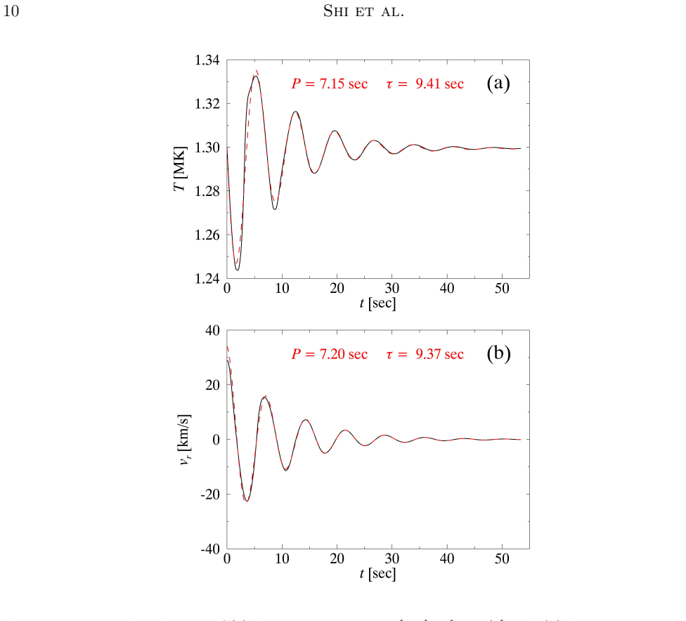
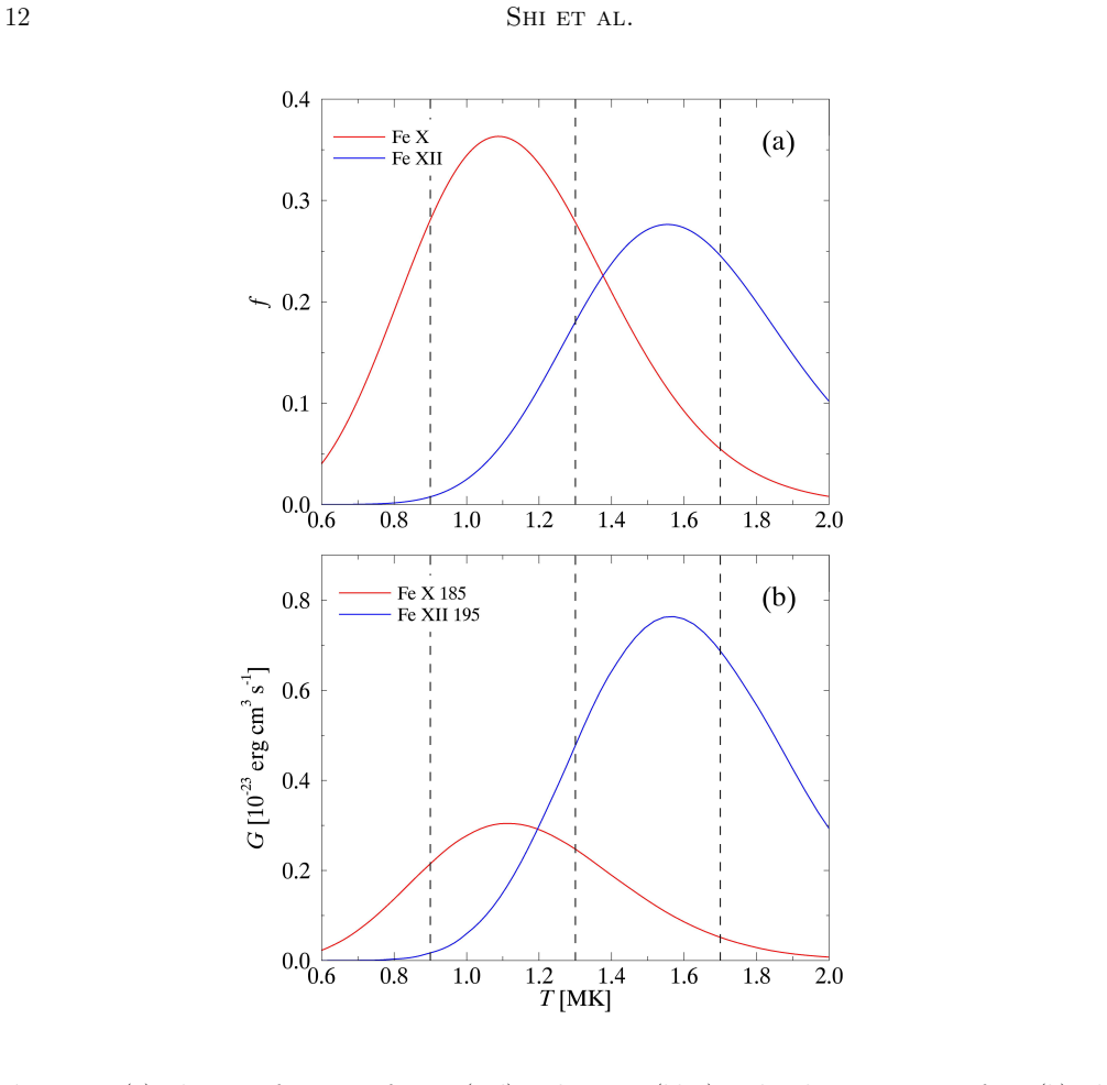
The load-bearing object is the first-order decomposition of the line intensity variation into a density term, $\Delta N \equiv 2N_0 \Delta N G_0$, and a contribution-function term, $\Delta G \equiv N_0^2 \Delta G$, whose ratio $R = (2/N_0)(dN/dT)/((1/G_0)(dG/dT))$ controls whether intensity and density oscillate in phase or anti-phase and how strongly the intensity decays. The damping time is then extracted by fitting an exponentially damped sinusoid to the crests and to the troughs of the synthesized intensity separately, and compared with the damping time obtained by fitting the same function to the transverse velocity from the magnetohydrodynamic simulation. Non-equilibrium ionization enters through the ionic fractions, which are evolved with the advective ionization-recombination equation rather than set to their temperature-dependent equilibrium values; this reduces the temperature sensitivity of the contribution function and makes the density term more dominant.

What would settle it

Observe a fast sausage mode in an active-region loop with a spectrometer capable of resolving several EUV lines, and measure both the intensity-derived damping time and the wave damping time independently, for instance from the transverse velocity or density oscillation. If, for a loop whose temperature is near the nominal formation temperature of the chosen line, the intensity-derived damping time consistently disagrees with the wave damping time by more than the few percent errors reported here, the central mapping would be ruled out. The sharpest test would be a loop at 0.9 MK observed in Fe XII 195 Å, where the model predicts a 41 percent overestimate of the damping time from the intensity crests.

Watch

Extended reading notes

Core claim

The central claim is that the damping time extracted from EUV intensity oscillations can serve as a faithful proxy for the damping time of leaky fast sausage modes, provided the loop temperature is close to the nominal formation temperature of the observed spectral line. The paper demonstrates this with numerical simulations of a standing leaky fast sausage mode in a straight cylindrical active-region loop, followed by forward synthesis of Fe X 185 Å and Fe XII 195 Å intensities. The mechanism is a competition between two first-order contributions to the intensity variation: one from density compression and one from the temperature sensitivity of the contribution function. Near the line's nominal formation temperature, the contribution-function term nearly vanishes, so intensity variations are dominated by density oscillations and their decay mirrors the wave's leakage-driven damping. When the loop is much hotter or cooler, the contribution-function term distorts the phase and amplitude of the intensity oscillation, so damping times from crests and troughs split and can deviate from the wave value, for example a 41 percent overestimate for Fe XII in a 0.9 MK loop.

Load-bearing premise

The entire argument assumes ideal magnetohydrodynamics, so the only source of wave damping is lateral leakage; if electron thermal conduction, proton viscosity, or heating/cooling misbalance damps the wave substantially in real active-region loops, the simulated damping times and the intensity-to-wave mapping will not carry over unchanged.

Editorial extensions

If this is right

If the claim is correct, EUV intensity oscillations from a suitably chosen spectral line can be used to measure the lateral-leakage damping time of fast sausage modes in active-region loops without resolving the loop.
The phase relation between density and intensity encodes whether the loop is near, above, or below the line's formation temperature, at least under equilibrium ionization.
Damping times from intensity crests and troughs can disagree substantially when the loop temperature is far from the formation temperature, so interpreting either alone would misestimate the wave damping time.
Non-equilibrium ionization changes the intensity amplitude but leaves Doppler velocity and Doppler width essentially unchanged, meaning spectral diagnostics are not a good alternative for extracting the period and damping of these modes.
The systematic dependence of the intensity-derived damping error on loop temperature means that observing multiple lines with different formation temperatures could jointly constrain the loop temperature and the wave damping time.

Reading between the lines

Editorial extensions of the paper, not claims the author makes directly.

An implication the paper leaves implicit is that the split between crest-derived and trough-derived damping times is itself a temperature diagnostic; a large asymmetry could flag that the observed line is not formed near the loop temperature.
Extending the same forward-modeling logic to other coronal lines with different formation temperatures should reproduce the same U-shaped error curve, so consistent multi-line damping estimates could triangulate the true loop temperature and wave damping time without additional spectroscopy.
Because real loops have thermal conduction, viscosity, and heating/cooling misbalance, a natural next test is to include those effects in the magnetohydrodynamic runs; if lateral leakage remains dominant, the temperature-matching recipe should survive, but if non-ideal damping dominates, the intensity-to-wave damping mapping will need revision.
The same decomposition applies to any strongly compressible wave that modulates density and temperature in phase, so the formation-temperature-matching rule may hold for slow magnetoacoustic waves and kink modes as well, provided their density-temperature phase relation is known.

Share X Bluesky LinkedIn Reddit HN

Signed reviews

No signed human review yet.

Editorial analysis

A structured set of objections, weighed in public.

Desk editor's note, referee report, and a circularity audit.

Desk Editor's Note

read the letter

This is the first forward-modeling study of leaky fast sausage modes in EUV emissions with non-equilibrium ionization, and it fills a real gap: earlier work, including the authors' own trapped-FSM papers, didn't cover the leaky regime. The central result—that the intensity-derived damping time tracks the wave damping time when the loop temperature is near the line's formation temperature—is supported by a clean systematic scan over loop temperature (Table 1, Figure 7). The first-order decomposition of density vs contribution-function terms in Section 3.1 is a nice piece of physics and makes the explanation convincing rather than hand-wavy. The paper is also honest about the ideal-MHD limitation, which is appropriate for a forward-modeling study.

The main soft spot is the fitting procedure. The paper computes damping times by fitting the crests and troughs of the intensity curve separately, then states the conclusion in terms of a single "damping time derived from the intensity." Observers—and anyone trying to use these results—will fit the full light curve with a damped sinusoid, not envelopes independently. The split-envelope method is fine for characterizing asymmetry, but it doesn't directly answer the question observers will ask. The qualitative conclusion likely survives: near the formation temperature, both crest and trough damping times are close to the wave value, so a full-signal fit would probably land in the same regime. But the quantitative errors in Table 1 (e.g., 41% vs -15.8% for Fe XII at 0.9 MK) show how much the two envelopes can diverge, and the paper doesn't report what a damped-sinusoid fit would give. That's a fixable but real gap.

The Doppler width and velocity conclusions rest on a single case and no noise or fit uncertainties, so those should be treated as preliminary. The ideal-MHD caveat is acknowledged and is not a hidden flaw.

Who is this for? Anyone doing coronal seismology with EUV spectroscopy, especially forward modeling of loop oscillations. It deserves a serious referee: the topic is relevant, the method is careful, and the core trend appears robust. My recommendation is to send it out. Before acceptance, the authors should add a damped-sinusoid fit to the synthetic intensity time series and report how the resulting damping time compares to the wave value; that would make the guidance genuinely operational.

Referee Report

3 major / 4 minor

Summary. The paper simulates standing leaky fast sausage modes (FSMs) in a straight cylindrical active-region loop using ideal MHD (PLUTO) for nine values of the loop-axis temperature Ti (0.9-1.7 MK). It then forward-models the Fe X 185 Å and Fe XII 195 Å emission with EIS-like spatial and spectral resolution, solving the ionization-recombination equations for non-equilibrium ionization (NEI). The intensity is integrated along a perpendicular line of sight through the loop apex, and damping times are extracted by fitting exponentials separately to the crests and troughs of the intensity time series. These intensity-derived damping times are compared with the wave damping time found from a fit to the MHD velocity perturbation. The central claim is that when Ti lies near the nominal formation temperature of the line, the intensity-derived damping time closely tracks the true leaky-FSM damping time, whereas for larger temperature deviations the discrepancy can be large (e.g., 41% for Fe XII at 0.9 MK). NEI is found to substantially modify the intensity variations but to have only marginal effects on Doppler velocity and width.

Significance. If the central claim holds, the paper provides a practical seismological proxy: EUV intensity damping measurements can be used to infer leaky-FSM damping times when the loop temperature is near the line formation temperature, with documented biases otherwise. The study's strengths include a systematic parameter scan over nine temperatures, a transparent first-order analytic decomposition of the intensity response in Section 3.1 (Eqs. 12-13), explicit NEI treatment via CHIANTI, and a self-consistency check between simulated fluid damping and forward-modeled intensity damping. The falsifiable trend in Figure 7 and Table 1 is a useful quantitative prediction for future high-cadence EUV spectroscopy. The authors also explicitly acknowledge that only ideal MHD is used, so the simulated damping is purely due to lateral leakage, and they discuss the potential role of thermal conduction, viscosity, and heating/cooling misbalance.

major comments (3)

[§3.2, Table 1, and Section 4] The central claim is phrased in terms of a single 'damping time derived from the intensity', but the paper only reports exponential fits performed separately on the crests and the troughs of the intensity envelope. An observer analyzing a real light curve would instead fit a damped sinusoid such as Equation (5) to the full time series. The manuscript does not report such a full-signal least-squares fit, nor does it argue that the crest/trough envelope procedure is equivalent to it. This leaves the main conclusion not operational for the measurement procedure actually used in observations. I request that the authors either add full-signal damped-sinusoid fits to the synthetic intensity time series for the NEI cases and report the resulting damping times, or explicitly restrict the claim to envelope-derived damping times and discuss how an observer should implement the recommended measurement.
[Table 1 and Figure 6] The exponential fits to the crests and troughs are reported without any uncertainties, even though the time series are short (of order a few oscillation periods before damping) and the crest/trough separation in some cases is large (e.g., Fe XII at Ti=0.9 MK gives 13.37 s from crests versus 7.98 s from troughs). Without confidence intervals or at least the number of fitted cycles, the quantitative relative errors in Table 1 and the apparent trend in Figure 7 cannot be fully assessed. The authors should provide fit uncertainties or state clearly how many cycles were used and why the differences are significant beyond the fitting noise.
[Section 3.1 and Section 4] The statement that NEI has only 'marginal effects' on the derived Doppler velocity or Doppler width is based on a single case: the Fe X 185 Å line for the base model (Ti=1.3 MK) with one specific line of sight (Figure 5). This is overgeneralized in the abstract and summary. The claim should either be restricted to the examined configuration or be supported by additional cases varying Ti and line choice.

minor comments (4)

[Section 3.1, around Eq. (12)] The notation in Equation (12) and the subsequent text uses ΔN to denote both the density perturbation and the first-order term 2 N0 ΔN G0, and similarly ΔG for the first-order term N0^2 ΔG. This is confusing; please rename the first-order terms (e.g., δN and δG) to avoid ambiguity.
[Table 1 caption] The caption contains the typo 'follwed' and the phrase 'displayed the damping times' should be 'display the damping times'. These are minor and can be corrected during revision.
[Abstract and Section 3.1] The abstract states that 'density variations and intensity variations can be either in phase or anti-phase' without specifying that this refers to the equilibrium ionization cases; in the NEI cases the behavior is described differently in Section 3.1. Please clarify this in the abstract for accuracy.
[Figure 7] The vertical dashed lines marking the nominal formation temperatures are helpful, but it would be clearer if the figure also identified which line each dashed line corresponds to, since the text says the lines are at 1.1 MK and 1.57 MK while the horizontal axis spans 0.9 to 1.7 MK.

Circularity Check

0 steps flagged · score 0.0 of 10

No significant circularity: the EUV damping times are forward-modeled from MHD simulations and compared with the wave damping times, with no fitted parameter forcing the agreement.

full rationale

The derivation chain is self-contained forward modeling. Section 2 computes the MHD fluid variables of leaky FSMs from the PLUTO ideal-MHD simulation, including the reference wave damping time from fitting v_r with Equation (5). Section 3 then synthesizes the line intensity from these simulated plasma states via I = integral(epsilon/4pi) dl with epsilon = G N^2, using CHIANTI contribution functions and solving the NEI ionization-recombination equations (Equations 6-9). The intensity damping times in Section 3.2 and Table 1 are extracted by exponential fits to the crests and troughs of the synthetic light curves and are then compared with the wave damping times. No parameter is fitted to the wave damping time, and no intensity damping value is inserted as an input; the comparison is an emergent test of whether the forward-modeled observable tracks the underlying wave damping. The near-agreement near the nominal formation temperature is explained by the relative sizes of the density and contribution-function first-order terms, Delta_N and Delta_G, in Equations (12)-(13), which is an analytic consequence of the simulation state rather than an assumed result. The self-citations (Shi et al. 2019a,b for the NEI framework; Chen et al. 2016, 2018 for boundary conditions and finite-beta effects) provide methodological setup and context, but the central claim rests on the present simulations and CHIANTI rates, not on an imported uniqueness theorem or ansatz. The final paragraph explicitly acknowledges that thermal conduction, viscosity, and heating/cooling misbalance are not modeled; this is a stated limitation about applicability to real loops, not a circular input. The skeptical concern that crest/trough fits differ from a full-signal damped-sinusoid fit is an operational question about how an observer would measure the damping time, not a circularity in the derivation. No self-definitional step, fitted-input-called-prediction step, or load-bearing self-citation chain exists in the paper.

Assumptions & free parameters 8 free parameters · 5 assumptions · 0 invented entities

The central claim depends on hand-chosen equilibrium and perturbation parameters, with Ti scanned but all other loop parameters fixed. It also depends on ideal-MHD modeling and on CHIANTI atomic data. No new physical entities are introduced. The damping-time comparison is a self-consistency check between two diagnostics of the same simulation, so the result is not a circular derivation but is not an independent observational test either.

free parameters (8)

Ti (loop axis electron temperature) = 0.9 to 1.7 MK in steps of 0.1 MK
Central trend in Figure 7 is parameterized by Ti; chosen by hand, not fitted to observations.
Interior and exterior electron densities Ni, Ne = 1e9 cm^-3 and 1e8 cm^-3
Sets the density contrast of 10, fixing the wave dispersion and the NEI response; only one contrast is tested.
Loop radius R0 = 2 Mm
Sets the spatial scale of the equilibrium and the leakage rate; not varied.
Density profile steepness delta = R0/4
Controls the width of the transverse density and temperature transition; chosen by hand.
Initial velocity perturbation amplitude a0 = 0.04 vAi
Sets the wave amplitude; amplitude-dependent effects are not explored.
Loop length L0 = 50 R0 (100 Mm)
Sets the longitudinal wavenumber k0 = pi/L0; only the fundamental standing mode is considered.
Magnetic field strengths Bi, Be = 10.87 G, 11.38 G
Fixed by pressure balance with the chosen density and temperature; affects wave speed and leakage.
Exterior temperature Te = 0.7 MK
Fixed exterior temperature; part of the equilibrium and affects the magnetic field profile.

assumptions (5)

domain assumption Ideal MHD with lateral leakage as the only damping mechanism adequately describes FSM evolution in active-region loops.
Section 2 uses the ideal MHD module of PLUTO; Section 4 lists thermal conduction, viscosity, and heating/cooling misbalance as unmodeled effects that could alter the wave and its emission.
domain assumption CHIANTI atomic data and ionization/recombination rate coefficients for Fe X and Fe XII are accurate.
Section 3 computes contribution functions and ionic fractions from CHIANTI; errors in rates propagate into the intensity and phase relations.
domain assumption At t=0 the plasma is in ionization equilibrium for the NEI initial condition.
Section 3 states the NEI solver is initialized with EI solutions for t=0; a prior non-equilibrium ionization state would change the temporal evolution of the ionic fractions.
domain assumption Along the perpendicular LoS, the intensity is dominated by the loop apex emissivity, I proportional to N^2 G.
Equation (12) in Section 3.1 uses apex values to explain the phase relations; column depth variations and off-apex contributions are neglected.
domain assumption Temperature and density perturbations at the loop apex are in phase for the simulated FSMs.
Used in Section 3.1 before Equation (13) to determine whether the density and contribution-function terms add or cancel.

how reviews work

0 comments

Cite this review

Pith. "Pith review of Synthetic Extreme-ultraviolet Emissions Modulated by Leaky Fast Sausage Modes in Solar Active Region Loops." pith.science (2026). https://pith.science/paper/DHPHDRYD

@misc{pith2026190807131,
  author       = {Pith},
  title        = {Pith review of: Synthetic Extreme-ultraviolet Emissions Modulated by Leaky Fast Sausage Modes in Solar Active Region Loops},
  year         = {2026},
  howpublished = {\url{https://pith.science/paper/DHPHDRYD}},
  note         = {Machine review of arXiv:1908.07131}
}

read the original abstract

We study the extreme-ultraviolet (EUV) emissions modulated by leaky fast sausage modes (FSMs) in solar active region loops and examine their observational signatures via spectrometers like EIS. After computing fluid variables of leaky FSMs with MHD simulations, we forward-model the intensity and spectral properties of the Fe X 185~\AA~and Fe XII 195~\AA~lines by incorporating non-equilibrium ionization (NEI) in the computations of the relevant ionic fractions. The damping times derived from the intensity variations are then compared with the wave values, namely the damping times directly found from our MHD simulations. Our results show that in the equilibrium ionization cases, the density variations and the intensity variations can be either in phase or in anti-phase, depending on the loop temperature. NEI considerably impacts the intensity variations but has only marginal effects on the derived Doppler velocity or Doppler width. We find that the damping time derived from the intensity can largely reflect the wave damping time if the loop temperature is not drastically different from the nominal formation temperature of the corresponding emission line. These results are helpful for understanding the modulations to the EUV emissions by leaky FSMs and hence helpful for identifying FSMs in solar active region loops.

Figures

Figures reproduced from arXiv: 1908.07131 by the authors.

**Figure 1.** Temporal evolutions of (a) the temperature T at [r, z] = [0, L0/2], and (b) the transverse velocity vr at [r, z] = [R0, L0/2] of leaky FSMs. The red dashed lines show the fitting curves from Equation (5), with the derived P and τ labeled in each panel. Here the base model is examined, i.e., the electron temperature at the loop axis Ti = 1.3 MK [PITH_FULL_IMAGE:figures/full_fig_p010_1.png] view at source ↗

**Figure 2.** Ionic fractions at the loop apex of Fe X (top) and Fe XII (bottom) versus time (left) and versus temperature (right). The red lines are for the equilibrium ionization (EI) cases while blue lines the non-EI cases. Here the base model is examined, i.e., the electron temperature at the loop axis Ti = 1.3 MK. An animation showing the trajectories is available online [PITH_FULL_IMAGE:figures/full_fig_p011_2.png] view at source ↗

**Figure 3.** (a) The ionic fractions of Fe X (red) and Fe XII (blue) under the assumption of EI. (b) The contribution functions G of Fe X 185 ˚A line (red) and Fe XII 195 ˚A line (blue) in the EI case. Three vertical dashed lines mark the temperatures of 0.9 MK, 1.3 MK, and 1.7 MK, respectively [PITH_FULL_IMAGE:figures/full_fig_p012_3.png] view at source ↗

Figures from the paper (4 more)

**Figure 4.** Figure 4: Temporal evolutions of the normalized intensity of Fe X 185 ˚A line (left) and Fe XII 195 ˚A line (right) for simulation cases with a number of values of Ti , the electron temperature at the loop axis. The LoS is perpendicular to the loop axis and passes through the lo…

**Figure 5.** Figure 5: Spectral profiles of the Fe X 185 ˚A line for EI and NEI cases. From top to bottom: spectral profiles Iλ, Doppler velocity vD, and Doppler width wD. The base model is examined, i.e., the electron temperature at the loop axis Ti = 1.3 MK. Here a different LoS is chosen.…

**Figure 6.** Figure 6: Exponential damping fits using the crests (red dashed lines) and the troughs (blue dashed lines) for the NEI intensity variations of (a) Fe X 185 ˚A with Ti = 1.3 MK, and (b) Fe XII 195 ˚A with Ti = 0.9 MK. The LoS is perpendicular to the loop axis and passes through t…

**Figure 7.** Figure 7: Relative errors of the damping time from the intensity variations with respect to the damping time of FSMs (see [PITH_FULL_IMAGE:figures/full_fig_p016_7.png]

Discussion (0). Continue with ORCID to comment.

Reference graph

Works this paper leans on

28 extracted references · 27 canonical work pages

[1]

2013, A&A, 555, A74

Antolin, P., & Van Doorsselaere, T. 2013, A&A, 555, A74

work page 2013
[2]

Melnikov, V. F. 2004, ApJ, 600, 458

work page 2004
[3]

2007, SoPh, 246, 3

Banerjee, D., Erd´ elyi, R., Oliver, R., & O’Shea, E. 2007, SoPh, 246, 3

work page 2007
[4]

Cally, P. S. 1986, SoPh, 103, 277

work page 1986
[5]

S., & Xiong, M

Cally, P. S., & Xiong, M. 2018, Journal of Physics A Mathematical General, 51, 025501

work page 2018
[6]

2018, ApJ, 855, 47

Chen, S.-X., Li, B., Kumar, S., Yu, H., & Shi, M. 2018, ApJ, 855, 47

work page 2018
[7]

2016, ApJ, 833, 114

Chen, S.-X., Li, B., Xiong, M., Yu, H., & Guo, M.-Z. 2016, ApJ, 833, 114

work page 2016
[8]

C., Nakariakov, V

Cooper, F. C., Nakariakov, V. M., & Williams, D. R. 2003, A&A, 409, 325 De Moortel, I., & Bradshaw, S. J. 2008, SoPh, 252, 101 De Moortel, I., & Nakariakov, V. M. 2012, Philosophical Transactions of the Royal Society of London Series A, 370, 3193 Del Zanna, G., Dere, K. P., Young, P. R., Landi, E., & Mason, H. E. 2015, A&A, 582, A56

work page 2003

Show all 28 references

[9]

M., & Roberts, B

Edwin, P. M., & Roberts, B. 1983, SoPh, 88, 179

1983
[10]

2012, A&A, 543, A12

Doorsselaere, T. 2012, A&A, 543, A12

2012
[11]

R., van Doorsselaere, T., Brady, C

Inglis, A. R., van Doorsselaere, T., Brady, C. S., & Nakariakov, V. M. 2009, A&A, 503, 569

2009
[12]

2018, ApJL, 855, L29

Kaneda, K., Misawa, H., Iwai, K., et al. 2018, ApJL, 855, L29

2018
[13]

Y., Nakariakov, V

Kolotkov, D. Y., Nakariakov, V. M., Kupriyanova, E. G., Ratcliﬀe, H., & Shibasaki, K. 2015, A&A, 574, A53

2015
[14]

Zavershinskii, D. I. 2019, arXiv e-prints, arXiv:1907.07051

2019 arXiv
[15]

G., Melnikov, A

Kopylova, Y. G., Melnikov, A. V., Stepanov, A. V., Tsap, Y. T., & Goldvarg, T. B. 2007, Astronomy Letters, 33, 706

2007
[16]

2018, SSRv, 214, 45

Dominique, M., Jel´ ınek, P., & Takasao, S. 2018, SSRv, 214, 45

2018
[17]

F., Reznikova, V

Melnikov, V. F., Reznikova, V. E., Shibasaki, K., & Nakariakov, V. M. 2005, A&A, 439, 727

2005
[18]

2007, ApJS, 170, 228

Mignone, A., Bodo, G., Massaglia, S., et al. 2007, ApJS, 170, 228

2007
[19]

M., & Melnikov, V

Nakariakov, V. M., & Melnikov, V. F. 2009, SSRv, 149, 119

2009
[20]

M., & Verwichte, E

Nakariakov, V. M., & Verwichte, E. 2005, Living Reviews in Solar Physics, 2, 3

2005
[21]

E., Antolin, P., & Van Doorsselaere, T

Reznikova, V. E., Antolin, P., & Van Doorsselaere, T. 2014, ApJ, 785, 86

2014
[22]

Schrijver, C. J. 2007, ApJL, 662, L119

2007
[23]

Spruit, H. C. 1982, SoPh, 75, 3

1982
[24]

T., Shen, Y

Su, J. T., Shen, Y. D., Liu, Y., Liu, Y., & Mao, X. J. 2012, ApJ, 755, 113

2012
[25]

R., Reeves, K

Tian, H., Young, P. R., Reeves, K. K., et al. 2016, ApJL, 823, L16 Van Doorsselaere, T., Antolin, P., Yuan, D.,

2016
[26]

M., Selzer, L

Yu, S., Nakariakov, V. M., Selzer, L. A., Tan, B., & Yan, Y. 2013, ApJ, 777, 159

2013
[27]

I., Kolotkov, D

Zavershinskii, D. I., Kolotkov, D. Y., Nakariakov, V. M., Molevich, N. E., & Ryashchikov, D. S. 2019, arXiv e-prints, arXiv:1907.08168

2019 arXiv
[28]

V., & Struminsky, A

Zimovets, I. V., & Struminsky, A. B. 2010, SoPh, 263, 163 10 Shi et al. Figure 1. Temporal evolutions of (a) the temperatureT at [r,z ] = [0,L 0/2], and (b) the transverse velocity vr at [r,z ] = [R0,L 0/2] of leaky FSMs. The red dashed lines show the ﬁtting curves from Equati...

2010

Pith tools

Reviewed August 14, 2026 · model on record in the stance chip above.

[1] [1]

2013, A&A, 555, A74

Antolin, P., & Van Doorsselaere, T. 2013, A&A, 555, A74

work page 2013

[2] [2]

Melnikov, V. F. 2004, ApJ, 600, 458

work page 2004

[3] [3]

2007, SoPh, 246, 3

Banerjee, D., Erd´ elyi, R., Oliver, R., & O’Shea, E. 2007, SoPh, 246, 3

work page 2007

[4] [4]

Cally, P. S. 1986, SoPh, 103, 277

work page 1986

[5] [5]

S., & Xiong, M

Cally, P. S., & Xiong, M. 2018, Journal of Physics A Mathematical General, 51, 025501

work page 2018

[6] [6]

2018, ApJ, 855, 47

Chen, S.-X., Li, B., Kumar, S., Yu, H., & Shi, M. 2018, ApJ, 855, 47

work page 2018

[7] [7]

2016, ApJ, 833, 114

Chen, S.-X., Li, B., Xiong, M., Yu, H., & Guo, M.-Z. 2016, ApJ, 833, 114

work page 2016

[8] [8]

C., Nakariakov, V

Cooper, F. C., Nakariakov, V. M., & Williams, D. R. 2003, A&A, 409, 325 De Moortel, I., & Bradshaw, S. J. 2008, SoPh, 252, 101 De Moortel, I., & Nakariakov, V. M. 2012, Philosophical Transactions of the Royal Society of London Series A, 370, 3193 Del Zanna, G., Dere, K. P., Young, P. R., Landi, E., & Mason, H. E. 2015, A&A, 582, A56

work page 2003