REVIEW 3 major objections 5 minor 29 references
A Prospective New Diagnostic Technique for Distinguishing Eruptive and Non-Eruptive Active Regions
T0 review · 3 major / 5 minor · reviewed 2026-08-14 · deepseek-v4-flash
Pith's one-line read A time-averaged magnetic force-balance metric, computed from magnetofrictional simulations of line-of-sight magnetograms, separates five eruptive from three non-eruptive active regions and is predictable 6 to 16 hours ahead.
desk verdict A physically motivated composite eruption metric with a nice spatial signal, but the 6–16 h forecast claim is in-sample and needs an out-of-sample test. read the letter →
The pith
A machine-rendered reading of the paper's core claim, the machinery that carries it, and where it could break.
The reading
What carries the argument
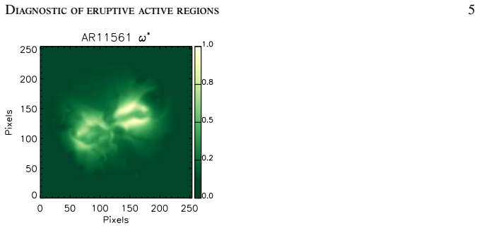
The load-bearing object is the eruption metric $\zeta=\omega\,\mu\,\sigma$ together with its time average $\bar{\zeta}$. $\omega$ accumulates a field-twist proxy $\Omega$ along the vertical direction to mark where flux ropes have formed; $\mu$ averages the height-integrated vertical Lorentz force in a small circular mask; $\sigma$ measures the spatial spread of that force in the same mask. Each factor is normalized by its running maximum and minimum so that different active regions can be compared, and the product stays between 0 and 1. The model that produces the underlying 3D field is a zero-$\beta$ magnetofrictional relaxation driven by a time series of line-of-sight magnetograms at the lower boundary, and the predictive test replaces the last observed magnetograms with a constant photospheric electric field deduced from the two most recent frames. The metric's work is to compress the entire simulated 3D force balance into a scalar that is elevated when a twisted structure, an outward force, and an unbalanced, heterogeneous force distribution coincide.
What would settle it
Run the same metric on a larger, independently classified sample of active regions and look at the distribution of $\bar{\zeta}$: if eruptive and non-eruptive populations overlap around 0.028, the threshold and the separation claim fail. A focused check would compare the modeled pre-eruptive Lorentz-force distribution against vector-magnetogram-based inference: a demonstrable mismatch between simulated and observed force balance would show that $\bar{\zeta}$ measures the model rather than the Sun.
Extended reading notes
Core claim
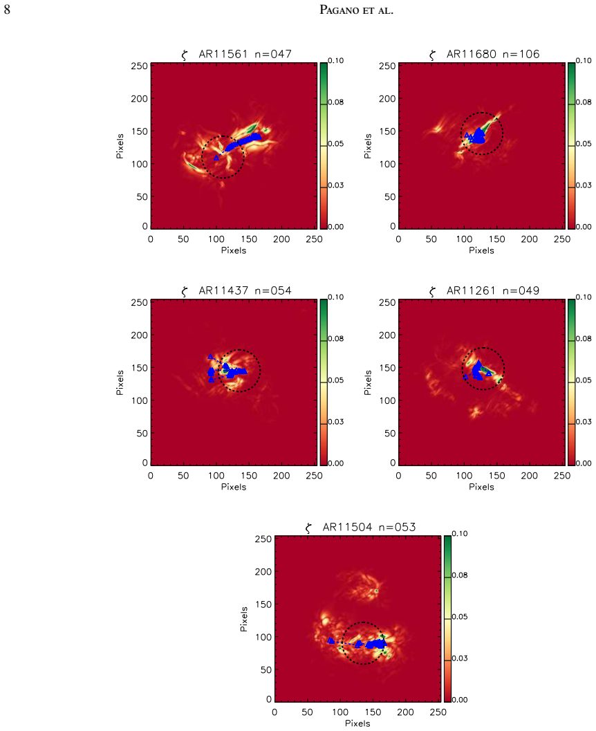
The central claim is that an active region's tendency to eject a flux rope can be read off one time-averaged quantity, $\bar{\zeta}$, computed from a magnetofrictional simulation of the coronal magnetic field. The instantaneous metric $\zeta(x,y,t)$ multiplies three normalized fields: $\omega$, a twist-based proxy for flux-rope formation; $\mu$, a vertically averaged outward Lorentz force; and $\sigma$, the local heterogeneity of that force. Taking the maximum of the spatially smoothed $\zeta$ over time and averaging after the initial ramp-up phase yields a value that is higher for the five eruptive regions than for the three non-eruptive ones; the paper sets a working threshold at $\bar{\zeta}_{\rm th}=0.028$. When the simulation is driven by projected magnetograms rather than observations, the final $\bar{\zeta}$ is reproduced when the projection starts within roughly ten magnetograms (about 16 hours) of the end of the series, with two regions needing a later start; adding random noise to the projected electric field does not change the classification. The paper also reports that the spatial location of high $\zeta$ coincides with the observed eruption site in four of the five eruptive cases.
Load-bearing premise
The diagnostic stands on the assumption that the simulated 3D coronal magnetic field is an accurate picture of the real pre-eruptive field, even though the simulation starts from a simplified potential-field state that the authors call an oversimplification.
Editorial extensions
If this is right
- A near-real-time pipeline could compute $\bar{\zeta}$ as each new magnetogram arrives and issue an alert when the threshold 0.028 is crossed, without needing eruption signatures to already be visible.
- Because the metric uses the full 3D force balance rather than photospheric maps alone, it offers something magnetogram-only parameters do not: a physical reason why one region is more pre-disposed to eject.
- For missions that must pick targets days in advance, the spatial map of $\zeta$ can point to the likely eruption site, not just the region, since the location of maximum $\zeta$ matched the observed eruption site in four of five cases.
- The insensitivity to random noise in the boundary electric field suggests the diagnostic can tolerate routine magnetogram errors and still separate classes.
Reading between the lines
- Inference: the two populations may overlap in a larger sample; the paper itself notes the within-group scatter exceeds the between-group gap, so the 0.028 threshold should be treated as a calibration point to re-fit rather than a universal constant.
- Inference: because the projection method keeps the boundary electric field constant, it systematically over-stresses regions undergoing flux emergence; a forecast-quality version would need a data-assimilated or decay-modeled boundary to extend lead times beyond 16 hours.
- Inference: comparing $\bar{\zeta}$ against decay-index or torus-instability calculations on the same simulated fields would test whether the metric tags the same pre-eruptive states as established instability criteria.
- Inference: the metric may be better suited to ranking eruption likelihood among many regions than to predicting exact onset, since the paper finds the eruption time does not always coincide with the maximum of $\zeta$.
Signed reviews
Editorial analysis
A structured set of objections, weighed in public.
Referee Report
Summary. The paper proposes a new diagnostic for distinguishing eruptive from non-eruptive solar active regions. The metric, ζ̄, is a time average of the maximum of a spatial product ζ = ω μ σ, where ω is a flux-rope proxy, μ is the vertically integrated Lorentz force, and σ is a Lorentz-force heterogeneity measure, all computed from NLFFF magnetofrictional simulations driven by line-of-sight magnetograms. The model is applied to eight previously studied active regions (five with observed eruption signatures, three without). The authors find that ζ̄ separates the two groups, set an empirical threshold ζ̄th = 0.028, and then run simulations in which the boundary magnetograms are projected forward from a cut-off time t0 to the final observed time tf, both with and without random-noise perturbations. They report that the threshold-based classification is reproduced for projections starting within about 16 hours (10 cadences) of tf and conclude that the metric provides a 'meaningful prediction' 6 to 16 hours in advance. The paper positions the technique as an initial step toward CME-onset forecasting and Solar Orbiter target selection.
Significance. If the claimed separation survived an out-of-sample or prospective test, this would be a valuable proof-of-concept: the metric is physically motivated, uses the full 3D coronal field rather than photospheric maps alone, and the projection experiments address a practical forecasting setup. The computational cost (under 1 hour on 16 cores per simulation), the potential for automation, and the explicit test with random boundary noise are strengths that partly offset the small sample. However, the current evidence does not establish predictive skill because the threshold is fitted to the same eight regions used for evaluation and the projection test is retrospective. The authors are transparent about the small sample and about the potential-field initial condition, but these caveats do not remove the need for an out-of-sample or chronological test before the headline claims are accepted.
major comments (3)
- [Sec. 3.5, Fig. 8] The threshold ζ̄th = 0.028 is defined as the average between the maximum non-eruptive ζ̄ and the minimum eruptive ζ̄ in the same eight-region sample, after the eruption labels are known. The separation between the two groups in Fig. 8 is therefore guaranteed by construction and cannot support the claim that the metric 'successfully differentiates' eruptive from non-eruptive regions in any predictive sense. No uncertainty or error bars are given for the ζ̄ values, and the authors themselves note that the within-population scatter exceeds the minimum between-population gap. The manuscript should either validate the threshold with leave-one-out cross-validation or on an independent sample, or explicitly reframe the claim as hypothesis-generating rather than as a confirmed diagnostic.
- [Sec. 4.2, Figs. 12–13] The forecast test is evaluated against a threshold calibrated on the full observed time series of the same active regions, so it does not simulate an operator who has only data up to t0. The forecast horizon is measured to tf, the end of the observed sequence, rather than to an independently defined eruption time; for AR11261 the eruption occurs about six minutes before tf, so runs with t0 = tf − 10Δt include in the threshold calibration the very outcome they are asked to predict. Moreover, for AR11261 and AR11437 the accurate reproduction of ζ̄ holds only for t0 ≥ tf − 5Δt, so the abstract's 6–16 hour window is not uniformly supported even by the in-sample metric. A prospective test would freeze the threshold and all normalization constants at t0, define the forecast target as an eruption occurring after t0, and measure skill separately for each lead time.
- [Sec. 5; Sec. 2.1] The physical content of ζ̄ depends entirely on the ability of the Mackay et al. (2011) magnetofrictional model to represent the quasi-static pre-eruptive coronal field, including the potential-field initial condition that the authors acknowledge in Sec. 5 is an oversimplification. Because the simulations are driven only by LOS magnetograms and assume zero-β quasi-static relaxation until a flux rope lifts off, the discrimination could be a property of the model's relaxation rather than of the Sun. This concern is not resolved by the noise experiments in Sec. 4.3, which test only perturbations of the boundary driver. I would like to see a sensitivity analysis (e.g., different initial conditions, different boundary-driving or relaxation parameters, or comparison with independent NLFFF codes) or a clear statement that the present claims are conditional on this modeling chain.
minor comments (5)
- [Sec. 3.5] The stated ramp-up time of 'around 35 magnetograms (between 40 and 55 hours)' is not consistent with the two cadences used: 35 × 60 min ≈ 35 h and 35 × 96 min ≈ 56 h; please clarify which cadence-dependent values are intended.
- [Fig. 8 caption] The caption calls ζ̄th = 0.028 a 'dashed curve', but the figure shows a horizontal dashed line; please correct the wording.
- [Reference list] The entry 'Yardley, S. L., Mackay, D. H., & Green. 2019, SoPh, 000, 0' is incomplete; please supply the full citation with volume and page or DOI.
- [Sec. 4.3] The noise-robustness test covers only two of the eight active regions, so the conclusion that the distinction is 'still maintained' should be restricted to these cases or supplemented by applying the noise test to the remaining regions.
- [Throughout] The manuscript contains several typographical errors, including 'buondary' in Sec. 4.1, 'consistence' in Sec. 3.4, and 'magentograms' in figure captions; a careful proofread is needed.
Circularity Check
The separation of eruptive and non-eruptive active regions is produced by a threshold fitted to the same eight regions it then classifies, and the 6–16 hour projection experiments are judged against that in-sample threshold, so the predictive claim is not independently tested.
-
fitted input called prediction
[Sec. 3.5 (threshold definition) and Fig. 8; abstract]
"For purely operational purposes, we compute a threshold of ¯ζth = 0.028, as the average between the maximum value of ¯ζ among the non-eruptive active regions and the minimum value of ¯ζ among the eruptive active regions (dashed horizontal line in Fig.8)."
The threshold is defined after the eruption labels are known, as the midpoint between the largest non-eruptive and smallest eruptive values in the same eight-region sample. Declaring that the metric "successfully differentiates active regions observed to produce eruptions from the non-eruptive ones in our data sample" is therefore a restatement of this construction: the separation is imposed by the choice of threshold, not discovered by an independent test. The paper itself notes the populations might overlap in a larger sample, but the in-sample discrimination claim is true by construction.
-
fitted input called prediction
[Sec. 4.2, Figs. 12–13; Conclusions]
"If we compare the value of ¯ζ to the threshold value ¯ζth, we find that for the majority of t0 ¯ζ remains larger than ¯ζth, indicating the possible occurrence of an eruption."
The projection experiments classify the same active regions used to set ¯ζth, and the threshold was calibrated on the full observed time series of those regions. The forecast horizon is measured to the final observed magnetogram tf, not to an independently defined eruption time, and the success criterion is agreement with the full-data simulation value rather than with held-out eruption labels. No cross-validated or out-of-sample evaluation is reported, so the claimed 6–16 hour predictive skill reduces to whether a projected curve stays on the fitted side of a boundary computed from the same events.
1 more flagged steps
-
other
[Sec. 4.2 (method of evaluation); Conclusions]
"To test the accuracy of the prediction we compared the final value of ¯ζ from these simulations that use projected magnetograms with the value found in the simulations that used the full sequence of observed magnetograms."
This explicitly defines prediction accuracy as agreement with the simulation driven by the complete observed magnetogram series of the same active region. Because ¯ζth is derived from exactly those full-data simulations, the evaluation cannot distinguish genuine anticipatory skill from the persistence of a fitted separator. The paper's own statements that the threshold is empirical and that larger samples may show overlap confirm that no independent validation is claimed here.
full rationale
The central discrimination claim is circular in the sense that the threshold is defined after the fact on the same data used to report success. The projection experiments likewise evaluate against the same fitted threshold and the reference simulations, so the reported 6–16 hour prediction horizon is not an out-of-sample test. The paper is transparent about the empirical nature of the threshold and the possibility of overlap in a larger sample, which is not a circularity defense but a limitation. However, the physical construct of zeta (flux-rope proxy, Lorentz force, heterogeneity) has independent content; the circularity lies solely in the evaluation protocol.
Assumptions & free parameters
free parameters (4)
- Eruption threshold zeta bar_th =
0.028
- Ramp-up cutoff =
35 magnetograms
- Smoothing scales (circular mask radius and square averaging size) =
0.7 Mm and 5.8 Mm
- Per-region normalization window =
cumulative min/max over t' <= t
assumptions (6)
- domain assumption The coronal magnetic field is well described by a zero-beta quasi-static force-free field, with magnetofrictional relaxation matching solar relaxation times.
- domain assumption The initial coronal field for each active region is potential.
- domain assumption Line-of-sight magnetograms at 96 or 60 minute cadence contain enough information to drive the 3D coronal field evolution.
- domain assumption Eruption labels taken from previous studies are correct and correspond to flux rope ejections.
- domain assumption After t0 the photospheric electric field remains constant in time.
- ad hoc to paper The threshold 0.028 estimated on eight regions generalizes to other active regions.
Cite this review
Pith. "Pith review of A Prospective New Diagnostic Technique for Distinguishing Eruptive and Non-Eruptive Active Regions." pith.science (2026). https://pith.science/paper/DU5F4VWR
@misc{pith2026190809223,
  author       = {Pith},
  title        = {Pith review of: A Prospective New Diagnostic Technique for Distinguishing Eruptive and Non-Eruptive Active Regions},
  year         = {2026},
  howpublished = {\url{https://pith.science/paper/DU5F4VWR}},
  note         = {Machine review of arXiv:1908.09223}
}
read the original abstract
Active regions are the source of the majority of magnetic flux rope ejections that become Coronal Mass Ejections (CMEs). To identify in advance which active regions will produce an ejection is key for both space weather prediction tools and future science missions such as Solar Orbiter. The aim of this study is to develop a new technique to identify which active regions are more likely to generate magnetic flux rope ejections. The new technique will aim to: (i) produce timely space weather warnings and (ii) open the way to a qualified selection of observational targets for space-borne instruments. We use a data-driven Non-linear Force-Free Field (NLFFF) model to describe the 3D evolution of the magnetic field of a set of active regions. We determine a metric to distinguish eruptive from non-eruptive active regions based on the Lorentz force. Furthermore, using a subset of the observed magnetograms, we run a series of simulations to test whether the time evolution of the metric can be predicted. The identified metric successfully differentiates active regions observed to produce eruptions from the non-eruptive ones in our data sample. A meaningful prediction of the metric can be made between 6 to 16 hours in advance. This initial study presents an interesting first step in the prediction of CME onset using only LOS magnetogram observations combined with NLFFF modelling. Future studies will address how to generalise the model such that it can be used in a more operational sense and for a variety of simulation approaches.
Figures


Figures from the paper (13 more)



Reference graph
Works this paper leans on
-
[1]
Amari, T., Luciani, J. F., Mikic, Z., & Linker, J. 2000, ApJL, 529, L49
work page 2000
-
[2]
Aulanier, G., T¨ or¨ ok, T., D´ emoulin, P ., & DeLuca, E. E. 2010, ApJ, 708, 314
work page 2010
-
[3]
Chen, P . F. 2011, Living Reviews in Solar Physics, 8, 1
work page 2011
- [4]
-
[5]
Florios, K., Kontogiannis, I., Park, S.-H., et al. 2018, SoP h, 293, 28
work page 2018
-
[6]
K., Bloomfield, D., Piana, M., et al
Georgoulis, M. K., Bloomfield, D., Piana, M., et al. 2017, AGU Fall Meeting Abstracts
work page 2017
-
[7]
Georgoulis, M. K., Massone, A. M., Jackson, D., et al. 2018, i n COSPAR Meeting, V ol. 42, 42nd COSPAR Scientific Assembly, PSW.1–11–18
work page 2018
-
[8]
Gibb, G. P . S., Mackay, D. H., Green, L. M., & Meyer, K. A. 2014, ApJ, 782, 71
work page 2014
Show all 29 references
-
[9]
2004, in ASSL V ol
Gopalswamy, N. 2004, in ASSL V ol. 317: The Sun and the Heliosphere as an Integrated System, ed. G. Poletto & S. T. Suess, 201– +
2004
-
[10]
M., Auch` ere, F., et al
Gopalswamy, N., Davila, J. M., Auch` ere, F., et al. 2011, in Proc. SPIE, V ol. 8148, Solar Physics and Space Weather Instrumentation IV , 81480Z 18 Pagano et al
2011
-
[11]
A., & DeForest, C
Howard, T. A., & DeForest, C. E. 2014, ApJ, 796, 33
2014
-
[12]
A., Forbes, T
Isenberg, P . A., Forbes, T. G., & Demoulin, P . 1993, ApJ, 417,368
1993
-
[13]
W., V alori, G., Green, L
James, A. W., V alori, G., Green, L. M., et al. 2018, ApJL, 855, L16
2018
-
[14]
2017, ApJ, 846, 106
Lowder, C., & Yeates, A. 2017, ApJ, 846, 106
2017
-
[15]
H., Green, L
Mackay, D. H., Green, L. M., & van Ballegooijen, A. 2011, ApJ, 729, 97
2011
-
[16]
H., & Yeates, A
Mackay, D. H., & Yeates, A. R. 2012, Living Reviews in Solar Physics, 9, 6
2012
-
[17]
H., Yeates, A
Mackay, D. H., Yeates, A. R., & Bocquet, F.-X. 2016, ApJ, 825, 131
2016
-
[18]
Ouyang, Y ., Yang, K., & Chen, P . F. 2015, ApJ, 815, 72
2015
-
[19]
H., & Poedts, S
Pagano, P ., Mackay, D. H., & Poedts, S. 2013a, A&A, 560, A38 —. 2013b, A&A, 554, A77 —. 2014, A&A, 568, A120
2014
-
[20]
H., & Yeates, A
Pagano, P ., Mackay, D. H., & Yeates, A. R. 2018, Journal of Spa ce Weather and Space Climate, 8, A26
2018
-
[21]
2017, SoPh, 292, 9 0
Rodkin, D., Goryaev, F., Pagano, P ., et al. 2017, SoPh, 292, 9 0
2017
-
[22]
J., Kauristie, K., Aylward, A
Schrijver, C. J., Kauristie, K., Aylward, A. D., et al. 2015, Advances in Space Research, 55, 2745
2015
-
[23]
Q., Zhang, J., Chen, Y ., & Cheng, X
Song, H. Q., Zhang, J., Chen, Y ., & Cheng, X. 2014, ApJL, 792, L40 T¨ or¨ ok, T., & Kliem, B. 2005, ApJL, 630, L97
2014
-
[24]
Wiegelmann, T., Petrie, G. J. D., & Riley, P . 2017, SSRv, 210, 249
2017
-
[25]
L., Jiang, C
Yan, X. L., Jiang, C. W., Xue, Z. K., et al. 2017, ApJ, 845, 18
2017
-
[26]
H., Sturrock, P
Yang, W. H., Sturrock, P . A., & Antiochos, S. K. 1986, ApJ, 309, 383
1986
-
[27]
L., Mackay, D
Yardley, S. L., Mackay, D. H., & Green. 2019, SoPh, 000, 0
2019
-
[28]
R., Attrill, G
Yeates, A. R., Attrill, G. D. R., Nandy, D., et al. 2010, ApJ, 7 09, 1238
2010
-
[29]
P ., Aulanier, G., & Gilchrist, S
Zuccarello, F. P ., Aulanier, G., & Gilchrist, S. A. 2015, ApJ , 814, 126
2015
Reviewed August 14, 2026 · model on record in the stance chip above.
Discussion (0). Continue with ORCID to comment.