REVIEW 3 major objections 6 minor 1 cited by
Chaos indicators for non-linear dynamics in circular particle accelerators
T0 review · 3 major / 6 minor · reviewed 2026-08-16 · deepseek-v4-flash
Pith's one-line read This paper establishes a power-law relation between stability time and Lyapunov time in a realistic LHC lattice, and argues that cheap chaos-indicator scans can replace long-term tracking for dynamic-aperture assessment.
desk verdict A solid exploratory application of FLIWB and REM to a realistic HL-LHC lattice, with a genuinely new TS–TL power-law observation whose extrapolation claim outruns the fit; worth refereeing, but the authors should be pushed to validate the extrapolation on censored and held-out data. read the letter →
The pith
A machine-rendered reading of the paper's core claim, the machinery that carries it, and where it could break.
The reading
What carries the argument
The load-bearing object is the empirical power law $T_S = \alpha T_L^{\beta}$ relating the first-passage stability time to the Lyapunov time, fitted to amplitude-binned averages in the weakly chaotic region. The Lyapunov time itself comes from FLIWB or REM: FLIWB uses a shadow particle whose displacement is renormalised every $\tau$ turns and weighted with Birkhoff averaging, while REM measures the distance after forward then backward tracking with round-off noise acting as the perturbation. A secondary mechanism is a Nekhoroshev-like formula $D(n)$ for the dynamic aperture as a function of the number of turns, which is fitted to both the $T_S$-based and $T_L$-based stability regions.
What would settle it
Take a magnetic-error seed not used in the fit, compute $T_L$ from FLIWB or REM at $10^6$ turns and $T_S$ from tracking to $10^7$ turns, bin by radial amplitude, and check whether $T_S = \alpha T_L^{\beta}$ with $\beta$ in [2,4] reproduces the data throughout the chaotic range; a clear deviation, or a threshold below which the log-log relation bends, would remove the extrapolation claim.
Extended reading notes
Core claim
This paper demonstrates that two fast chaos indicators, the Birkhoff-weighted Fast Lyapunov Indicator and the Reverse Error Method, can be applied to a realistic model of the high-luminosity LHC lattice, including synchrotron motion, and reproduce the phase-space structure that would otherwise require tracking up to $10^7$ turns. It establishes that the stability time $T_S$ and the Lyapunov time $T_L$ are related by a power law $T_S = \alpha T_L^{\beta}$ with $\beta$ between 2 and 4 across two magnetic-error seeds and three longitudinal amplitudes, and that a dynamic aperture defined through $T_L$ follows the same Nekhoroshev-like scaling law as the standard $T_S$-based aperture when longitudinal dynamics is present. The authors conclude that Lyapunov-based stability regions can stand in for conventional long-term dynamic-aperture estimates at a fraction of the computational cost, while cautioning that extrapolation of the power law requires further tests.
Load-bearing premise
The power-law relation is fitted on just two magnetic-error seeds and three longitudinal starting amplitudes, and it is assumed to keep holding for other error realisations, optics, energies, and configurations with beam-beam effects.
Editorial extensions
If this is right
- A dynamic aperture evaluated through Lyapunov time follows the same Nekhoroshev-like scaling as the standard stability-time aperture when longitudinal dynamics is present, so Lyapunov-based stability regions can substitute for conventional dynamic-aperture estimates.
- REM yields a sharper bimodal distribution of indicator values with a threshold that is nearly independent of the number of turns, enabling fast binary classification of regular and chaotic orbits in realistic lattices.
- FLIWB converges more rapidly than plain FLI for regular orbits, improving the separation between regular and chaotic initial conditions at fixed computational cost.
- The power law $T_S = \alpha T_L^{\beta}$ with $\beta \in [2,4]$ may provide extrapolation to higher stability times critical for lattice optimisation, subject to further validation across settings.
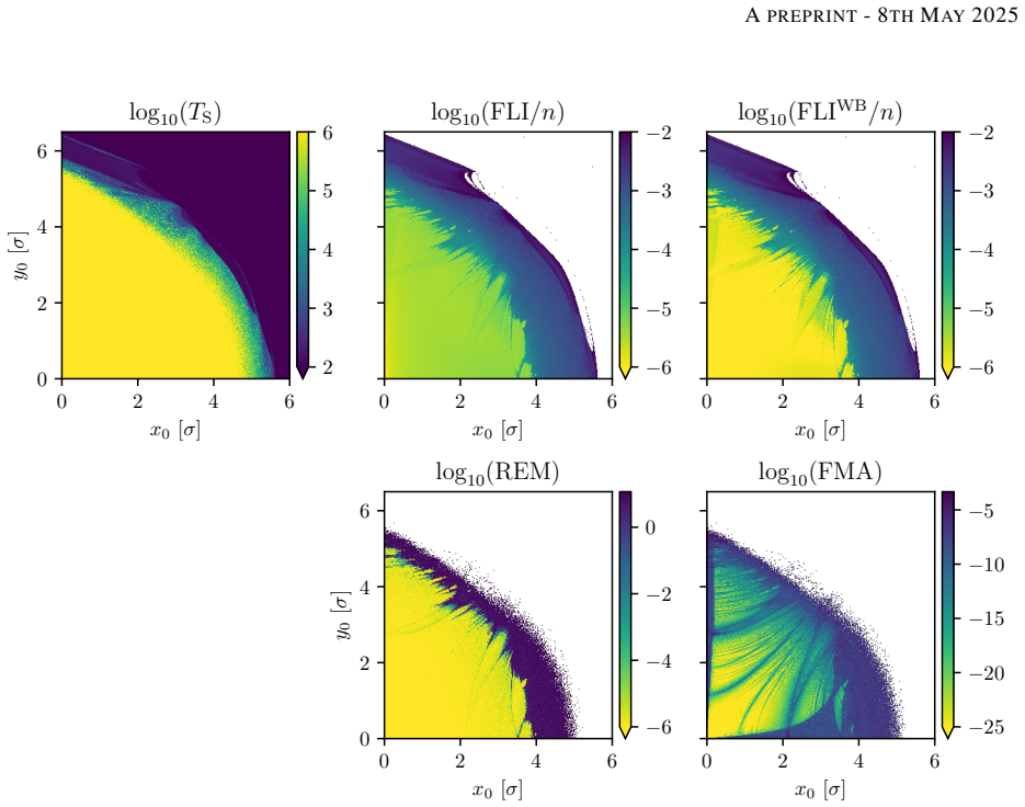
- Frequency Map Analysis is shown to be unreliable for locating chaotic regions when tune modulation from longitudinal dynamics is present, whereas FLIWB and REM remain informative.
Reading between the lines
- If the power-law extrapolation survives additional magnetic-error seeds, statistical screening of the many error realisations used in collider design becomes feasible: one-million-turn indicator maps could rank order stability across thousands of lattice variants.
- The diffusion reading of $\beta \in [2,4]$ suggests a testable link to beam-halo loss measurements: loss rates from collimator scans should match the action-diffusion coefficient inferred from Lyapunov-time maps.
- The same methodology should port to other storage rings where long tracking is prohibitive, but the paper's own caveat that no ground truth exists for realistic lattices means each new lattice needs a subsample cross-check against long tracking.
- A natural extension is to exploit REM's sharp bimodal distribution to set an automatic, iteration-independent chaos threshold and feed the resulting binary maps directly into an optimisation objective for tuning non-linear magnet families.
Signed reviews
Editorial analysis
A structured set of objections, weighed in public.
Referee Report
Summary. This paper applies the Birkhoff-weighted Fast Lyapunov Indicator (FLIWB) and the Reverse Error Method (REM) to realistic HL-LHC lattice models that include synchrotron motion, with the goal of assessing whether these indicators can serve as cheap proxies for long-term dynamic aperture (DA). The authors implement the indicators in the Xsuite GPU tracking code, study the influence of the shadow-particle parameters (initial displacement epsilon_0 and renormalization interval tau), and produce phase-space maps of stability time, FLIWB, REM, and FMA for two representative magnetic error seeds and three longitudinal amplitudes zeta_0. They then compare DA curves derived from stability time TS and Lyapunov time TL, fit a Nekhoroshev-type scaling law to both, and fit a power-law relation TS = alpha TL^beta to radially averaged data in an attempt to connect short-time chaos indicators to long-term stability. The central conclusion is that the power law may offer reliable extrapolation to high TS values and that TL-based stability regions could substitute for DA in lattice optimization.
Significance. If the extrapolation claim were valid, this would be a practically valuable way to reduce the cost of DA optimization in hadron colliders. The paper is solid in its descriptive content: it reports a careful implementation of FLIWB and REM within a modern GPU tracking framework, includes a parameter-sensitivity study, and is transparent about limitations (e.g., the absence of ground truth for chaotic regions acknowledged in Appendix B.3 and the explicit caveat in Section 4.2 on extrapolation). The numerical evidence, however, does not yet establish the central predictive claim. The power-law fit is conditional on escape within the tracking horizon, the parameters are largely unconstrained for zeta_0 = 0, and the Nekhoroshev-like scaling for TL-based DA fails for zeta_0 = 0. Thus the paper's main value lies in its demonstration of feasibility and in the phase-space maps, rather than in a validated extrapolation tool.
major comments (3)
- [4.2 and Fig. 8] The power-law fit TS = alpha TL^beta is restricted to initial conditions with TS < 10^7 turns, i.e., the 'white region' in Fig. 8, deliberately excluding all orbits that survive the full 10^7-turn tracking horizon. The extrapolation to higher TS values claimed in Section 5 concerns precisely the censored population (TS >= 10^7), yet the fit provides no information about the scaling of that population; the conditional distribution of TS given escape is not the same as the unconditional survival distribution. The text in Section 4.2 correctly identifies the bias and excludes the censored data 'to cope with this problem', but this procedure converts a censored-data problem into a selection-biased regression and does not resolve the issue. To support the extrapolation statement, the analysis would need to include the censored observations (e.g., via survival-analysis methods) or the conclusion should be explicitly limited to the range over which the fit is valid.
- [4.2 and Figs. 9-10] For the configuration closest to standard DA computations, zeta_0 = 0, the power-law fit parameters are effectively unconstrained: the worst seed yields log10(alpha) = -3 +/- 4 and beta = 2 +/- 2, and the best seed yields beta = 2.0 +/- 0.8. With a 100% relative uncertainty on beta, the data at zeta_0 = 0 cannot discriminate between the claimed beta in [2,4] and other scalings, so the statement that the action dynamics 'could have features compatible with diffusion regimes' is not supported by the reported fit in this case. Since zeta_0 = 0 corresponds to the case most relevant to conventional betatron-only dynamic aperture studies, the universality of the relation across all zeta_0 is not established.
- [Table 2 and Section 5] The conclusion in Section 5 that 'both measures follow a similar scaling law, effectively described by a Nekhoroshev-like scaling law' is not consistent with Table 2 for the TL-based DA in the zeta_0 = 0 rows, where the reduced chi-squared is chi2_nu = 4.7 (best seed) and 5.01 (worst seed), compared to chi2_nu = 0.03 for the TS-based fits. The model does not describe the TL-based DA data in the standard case without longitudinal coupling, and the text itself acknowledges that 'the quality of the fit is much worse for zeta_0 = 0'. The similar-scaling conclusion should either be restricted to the zeta_0 != 0 cases or the model's failure in the most relevant regime should be addressed before claiming substitutability of TL-based SR for DA.
minor comments (6)
- [Abstract] The phrase 'for the luminosity the beam lifetime optimisation' should read 'for the luminosity and the beam lifetime optimisation'.
- [Section 2.4] The sentence 'hence, for the reminder of this study' contains a typo; 'reminder' should be 'remainder'. The same typo appears later in the same section.
- [Appendix B.1] The phrase 'This arbitrarily threshold strategy' should be 'This arbitrary threshold strategy'.
- [Equation (1)] Equation (1) appears incorrectly typeset in the preprint (e.g., the '1h' following the multiplication sign and the broken exponent in the Lambert W expression), obscuring the definition of the DA model. The equation should be verified in the final version.
- [Section 4.2 and Fig. 7] The choice of Delta r = 0.01 sigma is described as the 'best compromise' between statistical fluctuations and information loss, but no quantitative criterion is stated; specifying the metric used would improve reproducibility.
- [Appendix B.3] Appendix B.3 correctly notes that no ground truth for chaotic regions is available for the realistic HL-LHC lattice; the wording in Section 3.1 that the indicators 'demonstrate the efficiency' in identifying chaotic dynamics should be tempered to reflect this acknowledged limitation.
Circularity Check
No circularity: TS and TL are measured independently, the power-law and DA scaling-law parameters are free fits, and the extrapolation caveat is a validity limitation rather than a self-referential construction.
full rationale
The paper's central quantitative claims are fits, not self-referential derivations. In Section 4.2, TS is obtained from tracking up to 1e7 turns to a control amplitude, while TL is obtained from FLIWB at 1e6 turns; these are different observables, and the power-law TS = alpha TL^beta has two free parameters fitted to binned averages. Nothing in the construction forces beta into [2,4]: the zeta0 = 0 cases give nearly unconstrained exponents (beta = 2 +- 2 for the worst seed and 2.0 +- 0.8 for the best seed), so the relation is not built in by definition. The DA scaling-law comparison in Section 4.1 is likewise a free-parameter fit (rho*, kappa) of Eq. (1) to each curve, with reduced chi-squared reported; calling the result 'described by a Nekhoroshev-like scaling law' is a goodness-of-fit statement, not a prediction extracted from the model's assumptions. The self-citations, chiefly [35] for indicator selection and [11] for the DA fitting form, supply a prior benchmark and a phenomenological ansatz; neither is invoked as an unverified uniqueness theorem that forbids alternatives, so self-citation is not load-bearing. The genuine weakness is acknowledged by the paper itself: Section 4.2 states that 'the power law's extrapolation abilities need further examination,' and the fit in Figs. 8-9 is restricted to the white region with TS < 1e7 turns, so the Section 5 claim of 'reliable extrapolation to higher TS values' is an unsupported empirical extrapolation, not a circular reduction. Appendix B.3 also concedes that 'it is not possible to establish a ground truth for the chaotic regions in the realistic HL-LHC lattice.' These caveats bear on validity and robustness, not on circularity by construction.
Assumptions & free parameters
free parameters (6)
- epsilon_0 (shadow particle initial displacement) =
1e-4 (chosen by convergence study)
- tau (renormalization interval) =
100 turns
- DA model parameters rho* and kappa =
Table 2: rho* 9.9-579, kappa 0.091-1.108 depending on seed and zeta0
- Power law parameters alpha and beta =
log10(alpha) -6.0 to -2.0, beta 2.0 to 3.5
- FLI threshold for regular/chaotic classification =
log10(FLI/n) = -4.5
- Radial bin width Delta r =
0.01 sigma
assumptions (6)
- domain assumption The single-particle dynamics of the HL-LHC lattice without beam-beam is well modeled by the MAD-X/Xsuite symplectic tracking.
- domain assumption The shadow-particle method accurately approximates the tangent map dynamics for the chosen epsilon_0 and tau.
- domain assumption Chaos can be inferred from positive maximum Lyapunov exponent estimated by FLIWB/REM at finite time.
- standard math The Nekhoroshev-like scaling law Eq. (1) with a Lambert W function is an appropriate model for DA evolution.
- domain assumption A power-law TS = alpha TL^beta relationship from the resonance-overlap regime [40] is assumed to apply to the HL-LHC lattice.
- domain assumption Orbits stable for 10^7 turns are treated as censored, and only those with TS < 10^7 are used in the fit.
Cite this review
Pith. "Pith review of Chaos indicators for non-linear dynamics in circular particle accelerators." pith.science (2026). https://pith.science/paper/EA3DJ7Y5
@misc{pith2026250412741,
  author       = {Pith},
  title        = {Pith review of: Chaos indicators for non-linear dynamics in circular particle accelerators},
  year         = {2026},
  howpublished = {\url{https://pith.science/paper/EA3DJ7Y5}},
  note         = {Machine review of arXiv:2504.12741}
}
read the original abstract
The understanding of non-linear effects in circular storage rings and colliders based on superconducting magnets is a key issue for the luminosity the beam lifetime optimisation. A detailed analysis of the multidimensional phase space requires a large computing effort when many variants of the magnetic lattice, representing the realisation of magnetic errors or configurations for performance optimisation, have to be considered. Dynamic indicators for chaos detection have proven to be very effective in finding and distinguishing the weakly-chaotic regions of phase space where diffusion takes place and regions that remain stable over time scales in the order of multiple hours of continuous operation. This paper explores the use of advanced chaos indicators, including the Fast Lyapunov Indicator with Birkhoff weights and the Reverse Error Method, in realistic lattice models for the CERN Large Hadron Collider (LHC). Their convergence, predictive power, and potential to define a magnetic lattice quality factor linked to long-term dynamic aperture are assessed. The results demonstrate the efficiency of these indicators in identifying chaotic dynamics, offering valuable insights of these chaos indicators for optimising accelerator lattices with reduced computational cost compared to the classical approach based on CPU-demanding long-term tracking campaigns.
Figures


Figures from the paper (13 more)




Forward citations
Cited by 1 Pith paper
-
Chaoticus: a parallel approach to the computation of chaos indicators
Chaoticus is a Python package that moves chaos indicator computations (SALI, GALI, Lagrangian descriptors, Lyapunov exponents) onto GPUs and claims order-of-magnitude speedups.
Reference graph
Works this paper leans on
-
[35]
A. Bazzani, M. Giovannozzi, C. E. Montanari, and G. Turchetti. Performance analysis of indicators of chaos for nonlinear dynamical systems. Phys. Rev. E, 107:064209, 6 2023
work page 2023
-
[1]
Panichi, L
F. Panichi, L. Ciotti, and G. Turchetti. Fidelity and reversibility in the restricted three body problem. Commu- nications in Nonlinear Science and Numerical Simulation, 35:53–68, 2016
2016
-
[2]
Panichi, K
F. Panichi, K. Go ´zdziewski and G. Turchetti. The reversibility error method (REM): a new, dynamical fast indicator for planetary dynamics. MNRAS, 468(1):469–491, 6 2017
2017
-
[3]
E. Lega, M. Guzzo, and C. Froeschl ´e. Theory and Applications of the Fast Lyapunov Indicator (FLI) Method. In C. Skokos, G. A. Gottwald, and J. Laskar, editors, Chaos Detection and Predictability, pages 35–54, Berlin, Heidelberg, 2016. Springer Berlin Heidelberg
2016
-
[4]
Guzzo and E
M. Guzzo and E. Lega. Theory and applications of fast lyapunov indicators to model problems of celestial mechanics. Celestial Mech. Dyn. Astron., 135(4):37, 2023
2023
-
[5]
Giovannozzi, W
M. Giovannozzi, W. Scandale, and E. Todesco. Prediction of long-term stability in large hadron colliders. Part. Accel., 56:195, 1997
1997
-
[6]
Hwang, C
K. Hwang, C. Mitchell, and R. Ryne. Rapidly converging chaos indicator for studying dynamic aperture in a storage ring with space charge. Phys. Rev. Accel. Beams, 23:084601, 8 2020
2020
-
[7]
Y . Li, Y . Hao, K. Hwang, R. Rainer, A. He, and A. Liu. Fast dynamic aperture optimization with forward-reversal integration. Nucl. Instrum. Methods Phys. Res., Sect. A, 988:164936, 2021
2021
Show all 90 references
-
[8]
Montanari, A
C.E. Montanari, A. Bazzani, M. Giovannozzi, and G. Turchetti. Using Dynamic Indicators for Probing Single- Particle Stability in Circular Accelerators. In Proc. IPAC’22, number 13 in International Particle Accelerator Conference, pages 168–171. JACoW Publishing, Geneva, Switze...
2022
-
[9]
Todesco and M
E. Todesco and M. Giovannozzi. Dynamic aperture estimates and phase-space distortions in nonlinear betatron motion. Phys. Rev. E, 53(4):4067–4076, 4 1996
1996
-
[10]
Giovannozzi, W
M. Giovannozzi, W. Scandale, and E. Todesco. Dynamic aperture extrapolation in presence of tune modulation. Phys. Rev., E57(3):3432, 3 1998
1998
-
[11]
Bazzani, M
A. Bazzani, M. Giovannozzi, E. H. Maclean, C. E. Montanari, F. F. Van der Veken, and W. Van Goethem. Advances on the modeling of the time evolution of dynamic aperture of hadron circular accelerators. Phys. Rev. Accel. Beams, 22:104003, 10 2019
2019
-
[12]
O. S. Br ¨uning, P. Collier, Ph. Lebrun, S. Myers, R. Ostojic, J. Poole, and P. Proudlock. LHC Design Report . CERN Yellow Reports: Monographs. CERN, Geneva, 2004
2004
-
[13]
Aberle, I B ´ejar Alonso, O Br¨uning, P Fessia, L Rossi, L Tavian, M Zerlauth, C
O. Aberle, I B ´ejar Alonso, O Br¨uning, P Fessia, L Rossi, L Tavian, M Zerlauth, C. Adorisio, A. Adraktas, M. Ady, J. Albertone, L. Alberty, M. Alcaide Leon, A. Alekou, D. Alesini, B. Almeida Ferreira, P. Alvarez Lopez, G. Am- brosio, P. Andreu Munoz, M. Anerella, D. Angal-Ka...
2025
-
[14]
Arduini, J
G. Arduini, J. Barranco, A. Bertarelli, N. Biancacci, R. Bruce, O. Br ¨uning, X. Buffat, Y . Cai, L.R. Carver, S. Fartoukh, M. Giovannozzi, G. Iadarola, K. Li, A. Lechner, L. Medina Medrano, E. M ´etral, Y . Nosochkov, Y . Papaphilippou, D. Pellegrini, T. Pieloni, J. Qiang, S....
2016
-
[15]
S. Das, Y . Saiki, E. Sander, and J. A. Yorke. Quantitative quasiperiodicity. Nonlinearity, 30(11):4111–4140, 10 2017
2017
-
[16]
Super convergence of ergodic averages for quasiperiodic orbits
Suddhasattwa Das and James A Yorke. Super convergence of ergodic averages for quasiperiodic orbits. Nonlin- earity, 31(2):491–501, 1 2018
2018
-
[17]
Panichi, L
F. Panichi, L. Ciotti and G. Turchetti. Fidelity and reversibility in the restricted three body problem. Commun. Nonlinear Sci. Numer. Simul., 35:53–68, 2016
2016
-
[18]
J. Laskar. Introduction to Frequency Map Analysis. In C. Sim ´o, editor, Hamiltonian Systems with Three or More Degrees of Freedom, pages 134 — 150, Dordrecht, 1999. Springer, Springer
1999
-
[19]
J. Laskar. Frequency map analysis and quasiperiodic decompositions. arXiv: Dynamical Systems, 2003
2003
-
[20]
J. Laskar. Frequency map analysis of an Hamiltonian system. In AIP conference proceedings, volume 344, pages 130–159. American Institute of Physics, 1995
1995
-
[21]
Lega and C
E. Lega and C. Froeschl ´e. Numerical investigations of the structure around an invariant KAM torus using the frequency map analysis. Physica D, 95(2):97–106, 1996
1996
-
[22]
Papaphilippou and J
Y . Papaphilippou and J. Laskar. Frequency map analysis and global dynamics in a galactic potential with two degrees of freedom. Astron. Astrophys., 307:427–449, 1996. 26 A PREPRINT - 8 TH MAY 2025
1996
-
[23]
Papaphilippou and J
Y . Papaphilippou and J. Laskar. Global dynamics of triaxial galactic models through frequency map analysis. Astron. Astrophys., 329:451–481, 1998
1998
-
[24]
Papaphilippou
Y . Papaphilippou. Global Dynamics of a Galactic Potential via Frequency Map Analysis. In C. Sim ´o, editor, Hamiltonian Systems with Three or More Degrees of Freedom, pages 523–527, Dordrecht, 1999. Springer Neth- erlands
1999
-
[25]
J. Laskar. Application of frequency map analysis. In The Chaotic Universe: Proceedings of the Second ICRA Network Workshop, Rome, Pescara, Italy, 1-5 February 1999, volume 10, page 115. World Scientific, 2000
1999
-
[26]
Comunian, A
M. Comunian, A. Pisent, A. Bazzani, G. Turchetti, and S. Rambaldi. Frequency map analysis of a three- dimensional particle in the core model of a high intensity linac. Phys. Rev. ST Accel. Beams , 4:124201, 12 2001
2001
-
[27]
J. Laskar. Frequency map analysis and particle accelerators. In Proceedings of the 2003 Particle Accelerator Conference, volume 1, pages 378–382 V ol.1, 2003
2003
-
[28]
Papaphilippou, L
Y . Papaphilippou, L. Farvacque, J. Laskar, and A. Ropert. Probing the Non-Linear Dynamics of the ESRF Storage Ring with Experimental Frequency Maps. In Proceedings of the 2003 Particle Accelerator Conference, volume 1, pages 3189–3191. IEEE, 2003
2003
-
[29]
Nadolski and J
L. Nadolski and J. Laskar. Review of single particle dynamics for third generation light sources through fre- quency map analysis. Phys. Rev. ST Accel. Beams, 6:114801, 11 2003
2003
-
[30]
Shun-Qiang, L
T. Shun-Qiang, L. Gui-Min, L. Hao-Hu, H. Jie, C. Guang-Ling, and W. Cheng-Lan. Nonlinear optimization of the modern synchrotron radiation storage ring based on frequency map analysis. Chinese Physics C, 33(2):127, 2009
2009
-
[31]
Shatilov, E
D. Shatilov, E. Levichev, E. Simonov, and M. Zobov. Application of frequency map analysis to beam-beam effects study in crab waist collision scheme. Phys. Rev. ST Accel. Beams, 14:014001, 1 2011
2011
-
[32]
Papaphilippou
Y . Papaphilippou. Detecting chaos in particle accelerators through the frequency map analysis method. Chaos, 24(2):024412, 2014
2014
-
[33]
Tydecks et al
T. Tydecks et al. FCC-ee Dynamic Aperture Studies and Frequency Map Analysis. In Proc. IPAC’18, pages 244–246. JACoW Publishing, Geneva, Switzerland, 2018
2018
-
[34]
Zisopoulos, Y
P. Zisopoulos, Y . Papaphilippou, and J. Laskar. Refined betatron tune measurements by mixing beam position data. Phys. Rev. Accel. Beams, 22:071002, 7 2019
2019
-
[36]
Bazzani, G
A. Bazzani, G. Servizi, E. Todesco, and G. Turchetti. A normal form approach to the theory of nonlinear betatronic motion. CERN Yellow Reports: Monographs. CERN, Geneva, 1994
1994
-
[37]
Bazzani, F
A. Bazzani, F. Brini, and G. Turchetti. Diffusion of the Adiabatic Invariant for Modulated Symplectic Maps.AIP Conf. Proc. 395, 129, 1997
1997
-
[38]
Bazzani, S
A. Bazzani, S. Siboni, and G. Turchetti. Diffusion in Hamiltonian systems with a small stochastic perturbation. Physica D, 76(1):8–21, 1994
1994
-
[39]
Froeschl ´e and E
C. Froeschl ´e and E. Lega. Weak chaos and diffusion in Hamiltonian systems. In The Dynamics of Small Bodies in the Solar System, pages 463–502. Springer, Berlin, Heidelberg, 1999
1999
-
[40]
Morbidelli and C
A. Morbidelli and C. Froeschl ´e. On the relationship between lyapunov times and macroscopic instability times. Celestial Mech. Dyn. Astron., 63(2):227–239, 6 1995
1995
-
[41]
Morbidelli and A
A. Morbidelli and A. Giorgilli. On a connection between KAM and Nekhoroshev’s theorems. Physica D , 86(3):514–516, 1995
1995
-
[42]
P. M. Cincotta, C. M. Giordano, and I. I. Shevchenko. Revisiting the relation between the lyapunov time and the instability time. Physica D, 430:133101, 2022
2022
-
[43]
Giovannozzi and E
M. Giovannozzi and E. McIntosh. Development of parallel codes for the study of nonlinear beam dynamics. Int. J. Mod. Phys. C, 8:155–170, 11 1996
1996
-
[44]
Ghorpade, J
J. Ghorpade, J. Parande, M. Kulkarni, and A. Bawaskar. GPGPU Processing in CUDA Architecture. CoRR, abs/1202.4347, 2012
2012 arXiv
-
[45]
Iadarola, R
G. Iadarola, R. De Maria, S. Lopaciuk, A. Abramov, X. Buffat, D. Demetriadou, L. Deniau, P. Hermes, P. Kicsiny, P. Kruyt, A. Latina, L. Mether, K. Paraschou, Sterbini, F. Van Der Veken, P. Belanger, P. Niedermayer, D. Di Croce, T. Pieloni, and L. Van Riesen-Haupt. Xsuite: an i...
2023
-
[46]
Iadarola
G. Iadarola. Xsuite documentation, 2022. https://xsuite.readthedocs.io
2022
-
[47]
De Maria, J
R. De Maria, J. Andersson, V .K. Berglyd Olsen, L. Field, M. Giovannozzi, P.D. Hermes, N. Høimyr, G. Iadarola, S. Kostoglou, E. H. Maclean, E. McIntosh, A. Mereghetti, J. Molson, D. Pellegrini, T. Persson, M. Schwinzerl, B. Dalena, T. Pugnat, I. Zacharov, and K.N. Sjobak. SixT...
2019
-
[48]
Pang and L
X. Pang and L. Rybarcyk. GPU accelerated online multi-particle beam dynamics simulator for ion linear particle accelerators. Comput. Phys. Commun., 185(3):744–753, 2014
2014
-
[49]
Oeftiger and S
A. Oeftiger and S. Hegglin. Space Charge Modules for PyHEADTAIL. In Proc. HB’16, pages 124–129. JACoW Publishing, Geneva, Switzerland, 2016
2016
-
[50]
Adelmann, P
A. Adelmann, P. Calvo, M. Frey, A. Gsell, U. Locans, C. Metzger-Kraus, N. Neveu, C. Rogers, S. Rus- sell, S. Sheehy, et al. OPAL a versatile tool for charged particle accelerator simulations. arXiv preprint arXiv:1905.06654, 2019
1905 arXiv
-
[51]
Schwinzerl, H
M. Schwinzerl, H. Bartosik, R. De Maria, G. Iadarola, A. Oeftiger, and K. Paraschou. Optimising and Extending a Single-Particle Tracking Library for High Parallel Performance. In Proc. IPAC’21, pages 4146–4149. JACoW Publishing, Geneva, Switzerland, 2021
2021
-
[52]
Hermes, R
P.D. Hermes, R. Bruce, R. De Maria, M. Giovannozzi, G. Iadarola, D. Mirarchi, and S. Redaelli. A Novel Tool for Beam Dynamics Studies with Hollow Electron Lenses. InProc. IPAC’22, number 13 in International Particle Accelerator Conference, pages 176–179. JACoW Publishing, Gene...
2022
-
[53]
Iliakis, H
K. Iliakis, H. Timko, S. Xydis, P. Tsapatsaris, and D. Soudris. Enabling Large Scale Simulations for Particle Accelerators. IEEE Trans. Parallel Distrib. Syst., 33(12):4425–4439, 2022
2022
-
[54]
van Riesen-Haupt et al
L. van Riesen-Haupt et al. Benchmarking equilibrium emittance simulation tools for the future circular collider. In Proc. IPAC’24, number 15 in IPAC’24 - 15th International Particle Accelerator Conference, pages 2461–2464. JACoW Publishing, Geneva, Switzerland, 05 2024
2024
-
[55]
Fornara et al
A. Fornara et al. Emittance growth studies due to crab cavity induced amplitude noise in the sps. In Proc. IPAC’24, number 15 in IPAC’24 - 15th International Particle Accelerator Conference, pages 3163–3166. JACoW Publishing, Geneva, Switzerland, 05 2024
2024
-
[56]
Ch. Skokos. The Lyapunov Characteristic Exponents and Their Computation. In J.-J. Souchay and R. Dvorak, ed- itors, Dynamics of Small Solar System Bodies and Exoplanets, pages 63–135, Berlin, Heidelberg, 2010. Springer Berlin Heidelberg
2010
-
[57]
Bartolini, A
R. Bartolini, A. Bazzani, M. Giovannozzi, W. Scandale, and E. Todesco. Tune evaluation in simulations and experiments. Part. Accel., 52:147–177. 29 p, 1995
1995
-
[58]
Bartolini, M
R. Bartolini, M. Giovannozzi, W. Scandale, A. Bazzani, and E. Todesco. Precise measurement of the betatron tune. Part. Accel., 55:1–10, 1996
1996
-
[59]
Russo, G
G. Russo, G. Franchetti, and M. Giovannozzi. New Techniques to Compute the Linear Tune. In Proc. IPAC’21, number 12 in International Particle Accelerator Conference, pages 4142–4145, Geneva, 08 2021. JACoW Pub- lishing, Geneva, Switzerland
2021
-
[60]
De Maria
R. De Maria. HL-LHC Optics v1.5 Update, 7 2019
2019
-
[61]
De Maria
R. De Maria. HL-LHC MAD-X optics V1.5 Tag v0.1, 1 2020
2020
-
[62]
https://mad.web.cern.ch/mad/
MAD - Methodical Accelerator Design. https://mad.web.cern.ch/mad/
-
[63]
Tancredi, A
G. Tancredi, A. S ´anchez, and F. Roig. A comparison between methods to compute lyapunov exponents. Astron. J., 121(2):1171, 2 2001
2001
-
[64]
A. N. Kolmogorov. On the Conservation of Conditionally Periodic Motions under Small Perturbation of the Hamiltonian. Dokl. Akad. Nauk SSR, 98:527, 1954
1954
-
[65]
J. Moser. On invariant curves of area-preserving mappings of an annulus. Nachr. Akad. Wiss. G¨ottingen Math.- Phys. Kl., II:1, 1962
1962
-
[66]
V .I. Arnold. Proof of a theorem of A.N. Kolmogorov on the preservation of conditionally periodic motions under a small perturbation of the Hamiltonian. Russ. Math. Surv., 18:9, 1963
1963
-
[67]
Nekhoroshev
N. Nekhoroshev. Behavior of Hamiltonian systems close to integrable. In Functional Analysis and Its Applica- tions, volume 5, page 338. Kluwer Academic Publishers-Plenum Publishers, 1971
1971
-
[68]
Nekhoroshev
N. Nekhoroshev. An exponential estimate of the time of stability of nearly-integrable Hamiltonian systems.Russ. Math. Surv., 32(6):1, 12 1977. 28 A PREPRINT - 8 TH MAY 2025
1977
-
[69]
Bazzani, S
A. Bazzani, S. Marmi, and G. Turchetti. Nekhoroshev estimate for isochronous non resonant symplectic maps. Cel. Mech., 47(4):333, 1990
1990
-
[70]
Turchetti
G. Turchetti. Nekhoroshev Stability Estimates for Symplectic Maps and Physical Applications. In J.-M. Luck, P. Moussa, and M. Waldschmidt, editors, Number Theory and Physics , volume 47 of Springer Proceedings in Physics, pages 223–234, Berlin, Heidelberg, 1990. Springer Berli...
1990
-
[71]
Giovannozzi
M. Giovannozzi. A proposed scaling law for intensity evolution in hadron storage rings based on dynamic aperture variation with time. Phys. Rev. ST Accel. Beams, 15:024001, 2 2012
2012
-
[72]
R. M. Corless, G. H. Gonnet, D. E. G. Hare, D. J. Jeffrey, and D. E. Knuth. On the lambertw function. Advances in Computational Mathematics, 5(1):329–359, 12 1996
1996
-
[73]
W. H. Press, S. A. Teukolsky, W. T. Vetterling, and B. P. Flannery. Numerical Recipes 3rd Edition: The Art of Scientific Computing. Cambridge University Press, USA, 3 edition, 2007
2007
-
[74]
Bazzani, M
A. Bazzani, M. Giovannozzi, and E. H. Maclean. Analysis of the non-linear beam dynamics at top energy for the CERN Large Hadron Collider by means of a diffusion model. Eur. Phys. J. Plus, 135(1):77, 2020
2020
-
[75]
C. E. Montanari, A. Bazzani, and M. Giovannozzi. Probing the diffusive behaviour of beam-halo dynamics in circular accelerators. Eur. Phys. J. Plus, 137(11):1264, 2022
2022
-
[76]
Montanari
C.E. Montanari. Diffusive approach for non-linear beam dynamics in a circular accelerator. Master thesis, Department of Physics and Astronomy, Alma Mater Studiorum – University of Bologna, 2019. CERN-THESIS- 2019-383
2019
-
[77]
C. E. Montanari, A. Bazzani, M. Giovannozzi, A. A. Gorzawski, and S. Redaelli. Testing the Global Diffusive Behaviour of Beam-Halo Dynamics at the CERN LHC Using Collimator Scans. InProc. IPAC’22, number 13 in International Particle Accelerator Conference, pages 172–175. JACoW...
2022
-
[78]
C. E. Montanari, R. B. Appleby, A. Bazzani, M. Giovannozzi, P. Hermes, A. Poyet, S. Redaelli, and G. Sterbini. Measurement of the nonlinear diffusion of the proton beam halo at the CERN LHC. Accepted for publication in Eur. Phys. J. Plus, 2025
2025
-
[79]
Milani and A
A. Milani and A. M. Nobili. An example of stable chaos in the solar system. Nature, 357(6379):569–571, 1992
1992
-
[80]
Milani, A
A. Milani, A. M. Nobili, and Z. Kne ˇzevi´c. Stable chaos in the asteroid belt. Icarus, 125(1):13–31, 1997
1997
-
[81]
Elaskar and E
S. Elaskar and E. del R ´ıo. Review of chaotic intermittency. Symmetry, 15(6), 2023
2023
-
[82]
C. H. Skokos, G. A Gottwald, and J. Laskar. Chaos detection and predictability, volume 1. Springer, 2016
2016
-
[83]
Froeschl ´e, R
C. Froeschl ´e, R. Gonczi, and E. Lega. The fast Lyapunov indicator: a simple tool to detect weak chaos. Applic- ation to the structure of the main asteroidal belt. Planetary and Space Science, 45(7):881–886, 1997. Asteroids, Comets, Meteors 1996 - II
1997
-
[84]
R. Barrio. Theory and Applications of the Orthogonal Fast Lyapunov Indicator (OFLI and OFLI2) Methods. Chaos Detection and Predictability, 915:55–92, 3 2016
2016
-
[85]
Panichi and G
F. Panichi and G. Turchetti. Lyapunov and reversibility errors for Hamiltonian flows. Chaos Solitons and Fractals, 112:83–91, 7 2018
2018
-
[86]
Turchetti and F
G. Turchetti and F. Panichi. Fast Indicators for Orbital Stability: A Survey on Lyapunov and Reversibility Errors. In C. G. Buzea, M. Agop, and L. Butler, editors, Progress in Relativity, chapter 10. IntechOpen, Rijeka, 2019
2019
-
[87]
IEEE Std 754-2019 (Revision of IEEE 754-2008) , pages 1–84, 2019
IEEE Standard for Floating-Point Arithmetic. IEEE Std 754-2019 (Revision of IEEE 754-2008) , pages 1–84, 2019
2019
-
[88]
P ¨oschel
J. P ¨oschel. The concept of integrability on cantor sets for Hamiltonian systems. Celestial Mech. Dyn. Astron., 28(1):133–139, 9 1982
1982
-
[89]
Laskar, C
J. Laskar, C. Froeschl ´e, and A. Celletti. The measure of chaos by the numerical analysis of the fundamental frequencies. Application to the standard mapping. Physica D, 56(2-3):253–269, 05 1992
1992
-
[90]
Bartolini and F
R. Bartolini and F. Schmidt. A computer code for frequency analysis of non-linear betatron motion. Technical report, CERN-SL-Note-98-017-AP, 1998. 29
1998
Reviewed August 16, 2026 · model on record in the stance chip above.
Discussion (0). Continue with ORCID to comment.