Picturesque convolution-like recurrences and partial sums' generation

Andrius Grigutis; Ignas Gasparavi\v{c}ius; Juozas Petkelis

REVIEW 3 major objections 6 minor 18 references

Picturesque convolution-like recurrences and partial sums' generation

T0 review · 3 major / 6 minor · reviewed 2026-08-06 · deepseek-v4-flash

Challenge this review Re-run · record.json Download PDF Read on arXiv ↗ Review JSON

Pith's one-line read The Riemann hypothesis is restated as convergence of a coefficient series.

desk verdict The generating-function framework is a solid, useful generalization, but the advertised Riemann hypothesis criterion is unproved and should be withdrawn or fully proved. read the letter →

arxiv 2507.23619 v1 pith:EBDJ7XYE submitted 2025-07-31 math.NT

Ignas Gasparavičius , Andrius Grigutis , Juozas Petkelis This is my paper · ORCID

classification math.NT MSC 11B3711M0630B1005A15

keywords convolution-likerecurrencelinearinitialvaluesMaclaurinseriespowerpartialsumsRiemannhypothesisgeneratingfunctions

topics The Riemann Hypothesis

open problems The Riemann Hypothesis

verification ladder T0 review T1 audit T2 compute T3 formal

The pith

A machine-rendered reading of the paper's core claim, the machinery that carries it, and where it could break.

The reading

The paper establishes a closed-form generating-function method for the convolution-like recurrence $a_n=\sum_{j=0}^{n+m} b_{n+m-j}a_j$ with a known complex sequence $b$, $b_0\ne 0$. The key consequence of Theorem 1 is the identity $G_{\alpha_k}(s)(B(s)-s^m)=\sum_{n=k}^{m-1} b_{n-k}s^n$, so each auxiliary sequence $\alpha_k$---and therefore every solution $a$---is read off from $B(s)$ by extracting coefficients. From this the authors derive when the limit $\lim_{n\to\infty} a_n$ exists, express the initial values $a_0,\dots,a_{m-1}$ back through that limit, and show that a suitable choice of $b$ makes $a$ many known sequences, including partial sums of $\zeta(a)$, $\pi$, and $e$. A final corollary claims that the Riemann hypothesis holds if and only if the coefficient series $\hat b_1+2\hat b_2+\cdots$ converges in the strip $1/2<\Re a<1$.

What carries the argument

The load-bearing object is the auxiliary sequence family $\alpha_0,\dots,\alpha_{m-1}$, each defined by the same recurrence (3) with unit initial vectors, together with their generating functions $G_{\alpha_k}(s)=\sum_{n=0}^\infty \alpha_k(n)s^n$. The identity that carries the argument is $G_{\alpha_k}(s)(B(s)-s^m)=\sum_{n=k}^{m-1} b_{n-k}s^n$, which makes every $\alpha_k$ the coefficient sequence of an explicitly known power-series quotient once $B(s)$ is known. This single identity yields the representation of arbitrary solutions, the Abelian limit theorem, the linear system in Theorem 3, and the selection of $b$ that produces famous partial sums.

What would settle it

Compute $\hat b_n(a)$ from Proposition 3 for several $a$ with $1/2<\Re a<1$ and numerically check convergence of $\sum_{j=1}^\infty j\hat b_j$; a single point where convergence disagrees with the zero-free status of $(2-2^{2-a})\zeta(a)$ would disprove Corollary 3. Concretely, finding a zero of $(2-2^{2-a})\zeta(a)$ in the strip at which the coefficient series converges would already settle it.

Watch

Extended reading notes

Core claim

The central discovery is that the recurrence (1) is coefficient extraction from a quotient, not a genuinely infinite problem. Writing $A(s)=\sum a_n s^n$ and $B(s)=\sum b_n s^n$, Theorem 1 proves $A(s)(B(s)-s^m)=\sum_{k=0}^{m-1}a_k\sum_{n=k}^{m-1}b_{n-k}s^n$, and for each basis sequence $\alpha_k$ the same manipulation gives $G_{\alpha_k}(s)(B(s)-s^m)=\sum_{n=k}^{m-1}b_{n-k}s^n$. Proposition 1 shows $a_n=\sum_{k=0}^{m-1}\alpha_k(n)a_k$, so the whole solution space is $m$-dimensional and explicitly generated. Theorem 2 gives a closed form for $\lim_{n\to\infty}\alpha_k(n)$ under the Abelian condition that the Maclaurin series of $(1-s)G_{\alpha_k}(s)$ converge at $s=1$, and when $\sum b_j=1$ and $m\ne\sum j b_j$ the limit equals $(\sum_{j=k}^{m-1}b_{j-k})/(m-\sum_{j=1}^\infty j b_j)$. Theorem 3 and Corollary 2 solve for the initial values from $\lim a_n$ via a linear system whose determinant is a Vandermonde-type product over the roots of $B(s)-s^m$. The applications choose $b$ so that $\alpha_0(n)$ is a prescribed partial sum: harmonic sums of $\zeta(a)$, Möbius-weighted sums, Hasse-type coefficients that evaluate $\zeta(a)$ in the whole plane, Leibniz sums for $\pi/4$, and exponential sums for $e$. From the Hasse-based choice the paper derives Corollary 3: the Riemann hypothesis is true exactly when $\hat b_1+2\hat b_2+\cdots$ converges in $1/2<\Re a<1$.

Load-bearing premise

The load-bearing premise is that convergence of the coefficient series $\hat b_1+2\hat b_2+\cdots$ in the strip is equivalent to the analytic function $(2-2^{2-a})\zeta(a)$ being zero-free there; the paper asserts this equivalence after Proposition 3 but does not prove it.

Editorial extensions

If this is right

Any solution of the recurrence can be computed by extracting coefficients from $B(s)$, bypassing step-by-step iteration of the recurrence.
When $\sum_j b_j=1$ and $m\ne\sum_j j b_j$, the limit $\lim_{n\to\infty} a_n$ is a finite rational expression in the first $m$ initial values and the known coefficients $b_j$.
The initial values $a_0,\ldots,a_{m-1}$ are recoverable from the single number $\lim_{n\to\infty}a_n$ by solving the linear system of Theorem 3, with explicit closed forms in Corollary 2.
Choosing $b$ appropriately generates many named sequences as $a$—Lucas, Bell, Catalan, Motzkin, Ramanujan tau, and the partial sums of $\zeta(a)$, $\pi$, and $e$.
If Corollary 3 holds, the Riemann hypothesis is equivalent to the convergence of $\hat b_1+2\hat b_2+\cdots$ on the strip $1/2<\Re a<1$.

Reading between the lines

Editorial extensions of the paper, not claims the author makes directly.

Inference: the same convolution inversion should apply to recurrences with a different shift or with an added forcing term, because the generating-function manipulation only uses the shift structure of the convolution.
Inference: for $m=1$, the construction gives a dictionary between sequences $b$ and sequences $a$: any sequence whose generating function $A(s)$ satisfies $A(s)(B(s)-s)=a_0 b_0$ is generatable, so the reachable sequences are exactly coefficients of reciprocals of power series of the form $B(s)-s$.
Inference: the equivalence in Corollary 3 can be probed numerically before any proof: if a point $a$ in the strip emerges where $\sum j\hat b_j$ diverges while $(2-2^{2-a})\zeta(a)$ is known to be nonvanishing, the corollary would be false; no such computation would, on its own, prove RH.
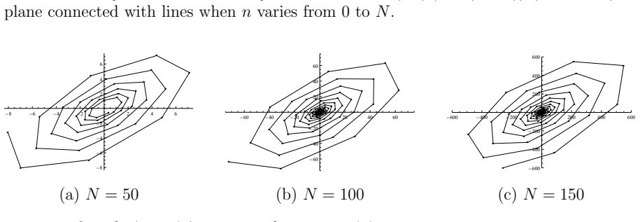
Inference: the paper's plots of $(\alpha_0(n),\alpha_0(n+1))$ track the radius of convergence of $G_{\alpha_0}$; the growth of successive coefficients in those plots should follow the reciprocal of the nearest singularity of $B(s)-s^m$, which Corollary 1 predicts.

Share X Bluesky LinkedIn Reddit HN

Editorial analysis

A structured set of objections, weighed in public.

Desk editor's note, referee report, and a circularity audit.

Desk Editor's Note

read the letter

Short version: the α-sequence generating-function framework is real and the extension from probability distributions to arbitrary b is useful, but Corollary 3's Riemann hypothesis criterion is not supported by the paper's own arguments. That advertised claim should be withdrawn until the missing analysis is supplied.

The core content is Theorem 1: the recurrence a_n = Σ b_{n+m−j} a_j is solved in closed form via (5)–(7). These are standard coefficient manipulations and they look correct. Generalizing the earlier m=2 probabilistic recurrences to general m and b with b0 ≠ 0 is natural and clean. The examples—Lucas, Catalan, Bell, Gould, and the partial-sum identities for ζ, π, e—are numerous, and the OEIS matches are a reasonable sanity check. For anyone working with convolution recurrences, this is a usable toolkit.

The soft spots sit in the Riemann hypothesis material. Proposition 3 is supposed to derive the generating function for the Hasse coefficients, but the proof says “After long and careful derivation (we omit details).” That means the central formula is not actually derived in the paper. Corollary 3 then claims RH is equivalent to convergence of Σ j b̂_j(a) in the strip. The stress-test note is right: the hypotheses of Proposition 3 (analyticity of f(s,a) in |s|<1 and lim f(s,a)=0 as s→1−) do not imply the ordinary coefficient series converges at s=1. That passage is a Tauberian step and no argument is supplied. So the RH criterion is an unproved equivalence, and it carries the full difficulty of RH. This does not undermine Theorem 1 or the examples, but it means the paper's most consequential statement should not be relied on.

There is also a self-containment issue: Theorem 3's determinant and Corollary 2's minors are imported from the authors' earlier paper [7] rather than proved here. That is acceptable if the citation holds up, but it makes the paper less independent. The plots are illustrative; missing error bars are a minor point for a math paper.

Who this is for: researchers in recurrences and generating functions, and readers who enjoy seeing famous sequences encoded as coefficients. The framework deserves a serious referee. My recommendation: send it to review, but require the authors either to give a complete proof of Proposition 3 and the convergence equivalence, or to delete Corollary 3 and the RH claims. The rest can stand alone.

Referee Report

3 major / 6 minor

Summary. The paper studies the convolution-like recurrence (1), a_n = sum_{j=0}^{n+m} b_{n+m-j} a_j, with known b and b_0 ≠ 0. It introduces m auxiliary sequences α_0,…,α_{m-1} so that a_n is a linear combination of a_0,…,a_{m-1} (Proposition 1), derives generating-function identities for these sequences (Theorem 1), gives conditions for the existence of limits and explicit limit formulas (Theorem 2), and provides a linear system for recovering a_0,…,a_{m-1} from lim a_n (Theorem 3 and Corollary 2). Propositions 2–4 construct sequences b whose α-sequences are partial sums of the Riemann zeta function, π/4, and e, and express the corresponding constants as ∑ j b_j. The most advertised consequence is Corollary 3, which states that the Riemann hypothesis is true if and only if ∑ j b̂_j(a) converges in 1/2 < Re a < 1 for the coefficients b̂_j of Proposition 3.

Significance. If the main framework is correct, Theorem 1 and Theorem 2 provide a clean, elementary generating-function method for solving a natural family of recurrences, and the OEIS examples in Section 4 give the paper a useful computational character. The direct coefficient manipulations in the proofs of Proposition 1 and Theorem 1 are plausible and accessible, and the limit formulas in Theorem 2 have the virtue of being explicit and checkable. However, the paper's most striking claim, the Riemann-hypothesis criterion in Corollary 3, is not supported by the arguments actually supplied: the step from a boundary value of a generating function to the ordinary convergence of the coefficient series is a nontrivial Tauberian statement, and the derivation of Proposition 3 is explicitly omitted. The paper therefore mixes a sound-looking core with an advertised result that is currently unproved.

major comments (3)

[§2, Corollary 3] Corollary 3 is not a consequence of the stated Proposition 3. Proposition 3 assumes that f(s,a) in (26) is analytic in |s|<1 and that lim_{s→1-} f(s,a)=0; under those hypotheses it derives the identity ζ(a)=1/((2-2^{2-a})(1-∑_{j≥1} j b̂_j(a))). The identity concerns the value at s=1 of a generating function, while the corollary concerns the ordinary convergence of the coefficient series ∑ j b̂_j(a). Passing from the former to the latter is a Tauberian step requiring coefficient estimates or a convergence theorem, and no such argument appears. Thus the equivalence 'RH iff ∑ j b̂_j(a) converges in 1/2<Re a<1' is currently an unsupported assertion, not a proved criterion.
[§3, Proof of Proposition 3] The proof of Proposition 3 consists of the sentence 'After long and careful derivation (we omit details)' followed by the claimed formal series B̂(s). Since B̂(s) defines the coefficients b̂_j on which Corollary 3 depends, this omission is load-bearing. The full derivation of B̂(s), including the identities for its coefficients, must be supplied in the manuscript or replaced by a complete reference with proof.
[§2, Theorem 3 and Corollary 2] Theorem 3's uniqueness claim rests on the determinant formula (30), which is cited from [7, Lem. 4.2] rather than proved, and Corollary 2's proof is deferred to [7, Proof of Thm. 3.3]. Because the invertibility of the system (17) is essential for the claimed inversion of initial values via lim a_n, the paper should either prove these determinant and minor identities or state the cited results in enough detail that the proof is self-contained. As written, a substantial part of the advertised inversion machinery lives in a previous paper.

minor comments (6)

[§2, Note 2 and Corollary 1] Note 2 refers to 'Corollary (1)' but the intended cross-reference is Corollary 1; the notation should be corrected.
[§3, proof of Theorem 1] The derivation of (9) from (28) equates coefficients of formal power series; the argument would be clearer if it explicitly stated that (28) is an identity of formal power series before invoking the Maclaurin expansion, since some of the displayed expressions are not known a priori to converge.
[§2, Proposition 2] In equation (25) the condition 'ℜα >1' appears at the end; this should be 'ℜa>1' as in the rest of the proposition.
[§4, Examples and figures] The figures in Section 2 and Section 4 are visually striking, but the axes are unlabeled and the plotted quantities are identified only in the captions; adding explicit axis labels and a short description of the plotted range would allow readers to verify the 'picturesque' patterns independently.
[§4.3, list of examples] The list of OEIS matches in §4.3 gives b sequences and the resulting a sequences without derivation or a proof that a = α_0 in each case; a sample derivation for at least two entries, plus a note on how the remaining entries are verified, would make the section reproducible.
[§2, Theorem 2] The condition 'b_0 + b_1 + … = 1' is used in (15) as if it were an ordinary convergent series, while elsewhere the paper works with formal power series; the analytic convergence assumptions should be stated explicitly in Theorem 2.

Circularity Check

0 steps flagged · score 0.0 of 10

No circular derivation chain found; Corollary 3 is underproved but not circular.

full rationale

The core derivation is a direct generating-function calculus. Theorem 1's identities (5)-(7) follow by multiplying recurrence (1) by powers of s and summing; the auxiliary sequences αk are defined independently in (3) and Table 1, so the result is not self-definitional. Propositions 2-4 are explicit constructions: the sequence b is chosen via its generating function so that α0(n) is a prescribed partial sum, and the identities connecting ∑ j bj with ζ, π, and e then follow from Theorem 2 together with external formulas (Hasse, Leibniz). These are verifications of a construction, not predictions fitted to the target. The only statement that might appear circular is Corollary 3, which rewrites the Riemann hypothesis as convergence of the series ∑ j \b j. However, the gap there is an omitted analytic/Tauberian proof, not a logical reduction: Proposition 3 states its hypotheses in terms of analyticity of f(s,a) and the limit at s→1, and the proof says 'After long and careful derivation (we omit details)'. Passing from the value of the generating function at s=1 to ordinary convergence of the coefficient series is a nontrivial step that is not supplied, but a missing justification is a correctness risk, not a circularity. The self-citations [7] and [9] are used for determinant computations and a probability limit result; they are separate published results and are not the load-bearing source of the generating-function identities. No step reduces by definition to its own input, so the paper is not circular.

Assumptions & free parameters 0 free parameters · 4 assumptions · 0 invented entities

The paper introduces no new physical or mathematical entities. Its free parameters are none: the sequence b is given or chosen, and the initial values a_0,...,a_{m-1} can be chosen freely. The main axiomatic dependencies are standard generating-function and complex-analysis facts, the external Hasse formula, and the authors' own earlier determinant results in [7].

assumptions (4)

domain assumption b0 is nonzero, so the recurrence can be rewritten as (2) and the auxiliary recurrences are well-defined.
This is a standing assumption in the abstract and in the statement of Theorem 1, and it is required to divide by b0 in equation (2) and in the initial table.
standard math The formal power series B(s), A(s), and G_alpha_k(s) are treated as formal objects, and the paper assumes Maclaurin series manipulations and analytic limits are valid where used.
Used throughout Sections 2 and 3, e.g. in Theorem 1, Corollary 1, and the proof of Theorem 2. No convergence issues are discussed for the formal series themselves.
standard math The Hasse formula (31) for the Riemann zeta function is used without proof.
Invoked in the proof of Proposition 3 to identify the limit of alpha_0 with (2 - 2^{2-a}) zeta(a). The formula is a known external result.
domain assumption Theorem 3 relies on the matrix determinant formula from the authors' earlier paper [7, Lem. 4.2], and Corollary 2 relies on [7, Proof of Thm. 3.3].
The determinant identity (30) and the minor computations used to prove equations (18)-(21) are not proved in this paper; they are imported from Grigutis [7].

how reviews work

0 comments

Cite this review

Pith. "Pith review of Picturesque convolution-like recurrences and partial sums' generation." pith.science (2026). https://pith.science/paper/EBDJ7XYE

@misc{pith2026250723619,
  author       = {Pith},
  title        = {Pith review of: Picturesque convolution-like recurrences and partial sums' generation},
  year         = {2026},
  howpublished = {\url{https://pith.science/paper/EBDJ7XYE}},
  note         = {Machine review of arXiv:2507.23619}
}

abstract

Let ${\pmb b}=\{b_0,\,b_1,\,\ldots\}$ be the known sequence of numbers such that $b_0\neq0$. In this work, we develop methods to find another sequence ${\pmb a}=\{a_0,\,a_1,\,\ldots\}$ that is related to ${\pmb b}$ as follows: $a_n=a_0\,b_{n+m}+a_1\,b_{n+m-1}+\ldots+a_{n+m}\,b_0$, $n\in\mathbb{N}\cup\{0\}$, $m\in\mathbb{N}$. We show the connection of $\lim_{n\to\infty}a_n$ with $a_0,\,a_1,\,\ldots,\,a_{m-1}$ and provide varied examples of finding the sequence ${\pmb a}$ when ${\pmb b}$ is given. We demonstrate that the sequences ${\pmb a}$ may exhibit pretty patterns in the plane or space. Also, we show that the properly chosen sequence ${\pmb b}$ may define ${\pmb a}$ as some famous sequences, such as the partial sums of the Riemann zeta function, etc.

Figures

Figures reproduced from arXiv: 2507.23619 by the authors.

**Figure 1.** b = {−3, 2, −1, 3, 0, 0, . . . , 0, . . .} and the pairs of (α0(n), α0(n+ 1)) in plane connected with lines when n varies from 0 to N. æ æ æ æ æ æ æ æ æ æ æ æ æ æ æ æ æ æ æ æ æ æ æ æ æ æ æ æ æ æ æ æ æ æ æ æ æ æ æ æ æ æ æ æ æ æ æ æ æ -0.4 -0.2 0.2 0.4 0.6 0.8 1.0 -0.4 -0.2 0.2 0.4 0.6 0.8 1.0 (a) N = 50 æ æ æ æ æ æ æ æ æ æ æ æ æ æ æ æ æ æ æ æ æ æ æ æ æ æ æ æ æ æ æ æ æ æ æ æ æ æ æ æ æ æ æ æ æ æ æ æ æ æ æ æ æ æ æ æ æ æ… view at source ↗

**Figure 2.** b = {3, −1, 0, 2, −3, 0, 0, . . . , 0, . . .} and the pairs of (α0(n), α0(n + 1)) in plane connected with lines when n varies from 0 to N. æ æ æ æ æ æ æ æ æ æ æ æ æ æ æ æ æ æ æ æ æ æ æ æ æ æ æ æ æ æ æ æ æ æ æ æ æ æ æ æ æ æ æ æ æ æ æ æ æ -0.5 0.5 1.0 1.5 2.0 -0.5 0.5 1.0 1.5 2.0 (a) N = 50 æ æ æ æ æ æ æ æ æ æ æ æ æ æ æ æ æ æ æ æ æ æ æ æ æ æ æ æ æ æ æ æ æ æ æ æ æ æ æ æ æ æ æ æ æ æ æ æ æ æ æ æ æ æ æ æ æ æ æ æ æ æ æ æ æ… view at source ↗

**Figure 3.** b = {3, 1, −3, −2, 2, 0, 0, . . . , 0, . . .} and the pairs of (α0(n), α0(n + 1)) in plane connected with lines when n varies from 0 to N. 11 [PITH_FULL_IMAGE:figures/full_fig_p011_3.png] view at source ↗

Figures from the paper (4 more)

**Figure 4.** Figure 4: b = {2, 0, 0, −3, 2, 0, 0, . . . , 0, . . .} and the pairs of (α0(n), α0(n+1)) in plane connected with lines when n varies from 0 to N. æ æ æ æ æ æ æ æ æ æ æ æ æ æ æ æ æ æ æ æ æ æ æ æ æ æ æ æ æ æ æ æ æ æ æ æ æ æ æ æ æ æ æ æ æ æ æ -5 5 10 -5 5 10 (a) N = 50 ææ ææææ æ æ …

**Figure 5.** Figure 5: b = {sin 1, sin 2, sin 3, . . .} and the pairs of (α0(n), α0(n + 1)) (in radians) in plane connected with lines when n varies from 0 to N. æ æ æ æ æ æ æ æ æ æ æ æ æ æ æ æ æ æ æ æ æ æ æ æ æ æ æ æ æ æ æ æ æ æ æ æ æ æ æ æ æ æ æ æ æ æ æ -8 -6 -4 -2 2 4 6 -8 -6 -4 -2 2 4 6 …

**Figure 6.** Figure 6: b = {F(n + 1)/φn , n ∈ N0}, where F(n) denotes the Fibonnaci number and φ is the golden ratio. We depict the pairs of (α0(n), α0(n + 1)) in plane connected with lines when n varies from 0 to N. 0 2 4 6 0 2 4 6 0 2 4 6 (a) N = 50 -20 0 20 40 -20 0 20 40 -50 0 50 (b) N =…

**Figure 7.** Figure 7: b = {3, 0, −3, −2, 3, 0, 0, . . . , 0, . . .}, and the triples of (α0(n), α0(n + 1), α0(n + 2)) in space connected with lines when n varies from 0 to N. 12 [PITH_FULL_IMAGE:figures/full_fig_p012_7.png]

Discussion (0). Continue with ORCID to comment.

Reference graph

Works this paper leans on

18 extracted references · 17 canonical work pages

[7]

Exact expression of ultimate time survival probability in homo- geneous discrete-time risk model

Andrius Grigutis. Exact expression of ultimate time survival probability in homo- geneous discrete-time risk model. AIMS Mathematics , 8(3):5181–5199, 2023

work page 2023
[1]

Lars V. Ahlfors. Complex Analysis: An Introduction to the Theory of Analytic Functions of One Complex Variable . McGraw-Hill, New York, 3rd edition, 1979

work page 1979
[2]

Boyer and Uta C

Carl B. Boyer and Uta C. Merzbach. A History of Mathematics . John Wiley & Sons, 2nd edition, 1991. Discussion of the Gregory–Leibniz series for π

work page 1991
[3]

Bi-seasonal discrete time risk model

Julius Damarackas and Jonas ˇSiaulys. Bi-seasonal discrete time risk model. Applied Mathematics and Computation , 247:930–940, 2014

work page 2014
[4]

Harold M. Edwards. Riemann ’s Zeta Function. Academic Press, New York and London, 1974. 28

work page 1974
[5]

Greene and Donald E

Daniel H. Greene and Donald E. Knuth. Mathematics for the Analysis of Algorithms. Birkh¨ auser, Boston, 3rd edition, 2007

work page 2007
[6]

Determining exact survival probability by setting discrete random variables in E

Andrius Grigutis. Determining exact survival probability by setting discrete random variables in E. Sparre Andersen’s model. Probability, Uncertainty and Quantitative Risk, 8(4):445–462, 2023

work page 2023
[8]

On 2 ×2 determinants originating from sur- vival probabilities in homogeneous discrete time risk model

Andrius Grigutis and Jonas Jankauskas. On 2 ×2 determinants originating from sur- vival probabilities in homogeneous discrete time risk model. Results in Mathematics, 77:204, 2022

work page 2022

Show all 18 references

[9]

The limit law of maximum of discrete partial- sums distribution

Andrius Grigutis and Artur Nakliuda. The limit law of maximum of discrete partial- sums distribution. Lithuanian Mathematical Journal , 64(4):481–490, 2024

2024
[10]

Ein summierungsverfahren f¨ ur die riemannscheζ-reihe

Helmut Hasse. Ein summierungsverfahren f¨ ur die riemannscheζ-reihe. Mathematis- che Zeitschrift , 32:458–464, 1930

1930
[11]

The On-Line Encyclopedia of Integer Sequences

OEIS Foundation Inc. The On-Line Encyclopedia of Integer Sequences. Published electronically at http://oeis.org, 2025

2025
[12]

Mathematica, Version 14.2

Wolfram Research, Inc. Mathematica, Version 14.2. Champaign, IL, 2024

2024
[13]

Noe and Jay V

Thomas D. Noe and Jay V. Post. Primes in Fibonacci n-step and Lucas n-step sequences. Journal of Integer Sequences , 8(4):Article 05.4.4, 2005

2005
[14]

Philippou and A

Andreas N. Philippou and A. A. Muwafi. Waiting for the kth consecutive success and the fibonacci sequence of order k. The Fibonacci Quarterly , 20(1):28–32, 1982

1982
[15]

Eric L. F. Roettger and Hugh C. Williams. Linear Recurrence Sequences, pages 171–183. Springer Nature Switzerland, Cham, 2025

2025
[16]

Applied Combinatorics

Alan Tucker. Applied Combinatorics. John Wiley & Sons, Hoboken, NJ, 5th edition, 2006

2006
[17]

The Penguin Dictionary of Curious and Interesting Numbers

David Wells. The Penguin Dictionary of Curious and Interesting Numbers . Penguin Books, London, revised edition, 1997

1997
[18]

Herbert S. Wilf. Generatingfunctionology. Academic Press, Boston, 3rd edition, 2005. 29

2005

Pith tools

Reviewed August 6, 2026 · model on record in the stance chip above.

[1] [7]

Exact expression of ultimate time survival probability in homo- geneous discrete-time risk model

Andrius Grigutis. Exact expression of ultimate time survival probability in homo- geneous discrete-time risk model. AIMS Mathematics , 8(3):5181–5199, 2023

work page 2023

[2] [1]

Lars V. Ahlfors. Complex Analysis: An Introduction to the Theory of Analytic Functions of One Complex Variable . McGraw-Hill, New York, 3rd edition, 1979

work page 1979

[3] [2]

Boyer and Uta C

Carl B. Boyer and Uta C. Merzbach. A History of Mathematics . John Wiley & Sons, 2nd edition, 1991. Discussion of the Gregory–Leibniz series for π

work page 1991

[4] [3]

Bi-seasonal discrete time risk model

Julius Damarackas and Jonas ˇSiaulys. Bi-seasonal discrete time risk model. Applied Mathematics and Computation , 247:930–940, 2014

work page 2014

[5] [4]

Harold M. Edwards. Riemann ’s Zeta Function. Academic Press, New York and London, 1974. 28

work page 1974

[6] [5]

Greene and Donald E

Daniel H. Greene and Donald E. Knuth. Mathematics for the Analysis of Algorithms. Birkh¨ auser, Boston, 3rd edition, 2007

work page 2007

[7] [6]

Determining exact survival probability by setting discrete random variables in E

Andrius Grigutis. Determining exact survival probability by setting discrete random variables in E. Sparre Andersen’s model. Probability, Uncertainty and Quantitative Risk, 8(4):445–462, 2023

work page 2023

[8] [8]

On 2 ×2 determinants originating from sur- vival probabilities in homogeneous discrete time risk model

Andrius Grigutis and Jonas Jankauskas. On 2 ×2 determinants originating from sur- vival probabilities in homogeneous discrete time risk model. Results in Mathematics, 77:204, 2022

work page 2022