REVIEW 4 major objections 4 minor 53 references
Modeling Long-Wavelength Amorphous Dust Emission Based on the Physically Motivated Soft-Potential Model
T0 review · 4 major / 4 minor · reviewed 2026-08-04 · deepseek-v4-flash
Pith's one-line read The soft-potential model fits the Perseus molecular cloud's far-infrared-to-microwave spectrum better than the two-level-systems model and unifies sub-mm flattening with anomalous microwave emission in one double-well potential.
desk verdict A careful transfer of the soft-potential model to dust emission with an honest SED fit, but the best-fit parameters sit outside the regime where the model was validated and the TLS comparison is not same-pipeline. read the letter →
The pith
A machine-rendered reading of the paper's core claim, the machinery that carries it, and where it could break.
The reading
What carries the argument
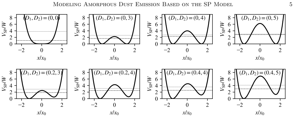
The quartic double-well potential V_SP(x) = W[D1(x/x0) - D2(x/x0)^2 + (x/x0)^4] is the central mechanism: the dimensionless D1 (asymmetry) and D2 (restoring force) set both the energy splitting epsilon of the lowest two levels and the barrier height V_b = W(D2/2)^2 in the analytical approximation, so the two previously independent TLS parameters become functions of one potential shape. The paper computes epsilon and the transition matrix element r12 directly from the Schrödinger equation (numerically) and via the standard tunneling approximation (analytically, with W, D1, D2 and approximations for Delta, Delta0, V_b, |r0|). The absorption cross-section is then assembled from three atom-level
What would settle it
Fit the SP model to a sample of molecular clouds covering a range of spectral indices and AME strengths, replacing the single Perseus fit. If the model cannot reproduce the low-beta, high-AME regions—where the soft-potential's low barriers should make hopping relaxation dominant—with a single parameter distribution, the central claim fails.
Extended reading notes
Core claim
Assuming that some atoms in amorphous dust are trapped in a double-well potential described by V_SP(x) = W[D1(x/x0) - D2(x/x0)^2 + (x/x0)^4], the author solves the Schrödinger equation directly—numerically and, under the standard tunneling approximation, analytically—to compute the electric-dipole transition matrix elements and the absorption cross-section. The discovery claimed is that the soft-potential model yields a self-consistent description of long-wavelength dust emission in which the level splitting epsilon and barrier height V_b both derive from the same D1, D2, W, eliminating the TLS model's treatment of them as independent. When fitted to the Perseus molecular cloud spectrum, the
Load-bearing premise
The claim rests on the assumed uniform distribution of double-well shapes f(D1,D2) = P_SP over a fixed domain cut off by Eqs. (37)-(39) with only the upper bound D_max2 free, a distribution with no independent support; the analytical best fit pins D_max2 at the imposed lower boundary D2 = 1.65, outside the D2 >= 4 region where the analytical approximation was validated.
Editorial extensions
If this is right
- If the SP model is correct, the anomalous microwave emission and the sub-millimeter spectral flattening are two manifestations of the same population of atoms in quartic double wells, so their intensities and frequency shapes should be correlated through the same D1, D2 distribution.
- The fitted low potential barriers mean hopping relaxation contributes significantly in the sub-millimeter, producing a smaller spectral index beta than the TLS model would predict for the same resonance intensity; the model may therefore succeed in low-beta regions where TLS struggles.
- The analytical approximate solution agrees with the numerical solution only for D2 ≳ 4; since the best-fit D_max2 for the Perseus cloud lies below that, accurate extraction of dust physical parameters from this model requires the numerical solution.
- Best-fit values for the energy scale W (~0.3 K), maximum splitting (Δ0/kB ~ 0.6 K), and number of trapped atoms per unit mass (~10^22 g^-1) fall orders of magnitude away from typical laboratory values for amorphous materials, so the model's parameters cannot be reconciled with current lab data unless interstellar dust differs strongly in composition or structure.
- The conversion formulas the paper derives show that the TLS model cannot be made to match the SP model simply by replacing its distribution functions; the SP model must be computed directly.
Reading between the lines
- If the SP model is right, a targeted multi-cloud survey that fits the model to regions with low beta and high AME should find that both features intensify together; the present paper fits only the Perseus cloud, so this correlation is a direct, testable prediction.
- The assumption of a uniform distribution f(D1,D2) is likely the soft spot; molecular dynamics simulations of amorphous silicates could in principle provide a first-principles distribution, and any deviation would shift the resonant band peak near epsilon/W ~ 2.1 and change the AME spectrum.
- The intermediate value of the CMB temperature fluctuation estimated from the SP model (-5 to -4 uK) versus TLS (-19 uK) and spinning dust (+23 uK) suggests that dust-model choice could bias low-level CMB foreground estimates in diffuse regions; this is an implication the author raises but does not pursue.
- A stronger test separating SP from spinning-dust AME: the SP model predicts AME from large grains should correlate with dust temperature (resonance transitions strengthen with T), whereas spinning-dust AME should correlate with the abundance of very small grains; the author points to this but does not carry out the correlation analysis.
Editorial analysis
A structured set of objections, weighed in public.
Referee Report
Summary. The paper applies the soft-potential (SP) model from amorphous-solid physics to interstellar dust emission. It assumes atoms are trapped in a quartic double-well potential, solves the Schr\"odinger equation numerically and with the standard tunneling approximation, and derives absorption cross-sections from the Bloch equations. The model is fitted to the Perseus molecular cloud SED from microwave to FIR, with reported reduced chi-square values of 1.33 (analytical) and 1.29 (numerical) versus 1.67 quoted for the TLS model. The authors claim that the SP model reproduces the observed spectrum slightly better than TLS and that the sub-mm flattening and AME share a single microscopic origin. The paper is explicit about the main limitations: the best-fit D_max2 lies outside the validated analytical regime, and the fitted physical parameters disagree with laboratory values by orders of magnitude.
Significance. If the central claim holds, the SP model would be a conceptual improvement over the TLS model: it derives the energy splitting and barrier height from one quartic potential rather than treating them as independent, and it connects the sub-mm spectral flattening (hopping relaxation) with the AME (resonant transitions). The derivation in Secs. 2\u20133 is careful, and the documented numerical-versus-analytical agreement for D2 \u2273 4 (Figs. 2\u20135) is a genuine strength. The paper is also honest about its caveats, including the D_max2 regime and the laboratory discrepancies in Table 3. However, the observational claim is currently a fit, not a prediction, and the fit depends on an assumed uniform parameter distribution and on low-D2 shapes for which the analytical solution was not validated. The modest chi-square improvement over TLS does not by itself establish the model, especially without a same-pipeline TLS refit or release of code/data. The contribution is promising but not yet conclusive.
major comments (4)
- [Sec. 2.5 / Table 2] The analytical SP solution is validated only for D2 \u2273 4 (Figs. 2\u20133, Sec. 2.5.1), yet the best-fit D_max2 = 1.65 (analytical, pinned at the Eq. (38) lower bound) and D_max2 = 2.11 (numerical) lie below this regime. The paper's own Sec. 6, item 2, concedes that the analytical solution is outside its scope. Because the resonance/AME band is produced by the \u03b5-distribution peaking near \u03b5/W \u2248 2.1 (Fig. 6), which is populated mainly by low-D2 shapes, the Perseus fit is not a test of the validated SP solution. Please validate or quantify the error of both solutions for 1.65 \u2264 D2 \u2264 4, and show that the fit is not an artifact of the imposed lower cutoff.
- [Sec. 3.2, Eqs. (36)–(39)] The uniform distribution f(D1,D2) = P_SP and the cutoffs (D1 \u2265 0, D2 \u2265 1.65, \u03b5 \u2264 \u03b5_max, with a free upper D_max2) are assumed with no independent physical justification. The AME band position is set by the \u03b5-distribution peak near \u03b5/W \u2248 2.1, so changing the distribution shape or the cutoff changes the resonance spectrum and the fitted SED. The paper does not provide a sensitivity analysis or a derivation of uniformity. Please test alternative distribution shapes/cutoffs, fit D_max2 as a genuinely free upper boundary rather than as an enforced lower boundary, and check whether the 10\u2013100 GHz fit survives such variations.
- [Sec. 5.2, Table 3] The best-fit physical parameters differ from laboratory values by 1\u20136 orders of magnitude: W, \u0394_max0, \u0394_min0, \u03b3, and N_DWP/(\u03c1V). The caveat that laboratory materials differ from interstellar dust is reasonable but does not resolve the tension, particularly f_SP \u2248 95% (analytical) or 59% (numerical), which implies that most atoms are in double-well potentials, far above typical laboratory DWP densities of 10^16\u201310^17 g^-1. For a model advertised as physically motivated, these fitted values undercut the physical interpretation. Please explore parameter degeneracies or correlations, impose laboratory constraints as priors, or provide an independent microscopic check.
- [Sec. 4, Fig. 8 / Table 2] The claimed improvement over TLS is based on \u03c7^2_red = 1.67 from Nashimoto et al. (2020a), not on a same-pipeline refit with identical data, identical components, and identical fitting code. With \u0394\u03c7^2_red \u2248 0.3\u20130.4, differences in the fitting setup, data selection, or nuisance-component treatment could easily dominate. Please refit the TLS model with the same data, same DCD model, and same free-free/CMB components, and report both \u03c7^2 and best-fit parameters. Releasing the fitting code and data would also make the comparison reproducible.
minor comments (4)
- [Eq. (24)] The definition of V_b is ambiguous as typeset. It should be V_b = V(x_O) - [V(x_L)+V(x_R)]/2 to match Eq. (27) and the usual barrier-height definition.
- [Fig. 7 caption] The caption says 'From the top, \u03b3, W, D_max2, and T', but the figure has a row/column layout with multiple curves. Please specify the panel arrangement explicitly.
- [Sec. 5.1.2, Eqs. (49)–(52)] The notation P0/P_SP and the Jacobian mapping between f(D1,D2) and f(\u0394,\u03940) need a clearer statement of units and normalization. As written, the reader must reconstruct the derivation to check consistency.
- [General] No data availability or code availability statement is provided. Given the number of fitting steps and the comparison with previous TLS fits, releasing the model code and the processed Perseus data would substantially strengthen reproducibility.
Circularity Check
No significant circularity: the SP cross-section is derived from the Schrödinger equation and Bloch equations, and the Perseus comparison is a fit to external data.
full rationale
The central derivation is self-contained: the absorption cross-section follows from solving the Schrödinger equation for a quartic double-well potential (Sec. 2.3), using the Bloch equations for the electric-field interaction (Sec. 2.2), and integrating over an assumed distribution f(D1,D2)=P_SP (Sec. 3.2). The observed Perseus spectrum enters only at the fitting stage (Sec. 4), not in the derivation of the cross-section. The claim that the SP model 'can reproduce' the Perseus SED is a goodness-of-fit statement against external data (Génova-Santos et al. 2015, Planck, WMAP, etc.), not a prediction derived from the model by construction. The sub-mm flattening and AME are attributed to specific terms (hopping/tunneling relaxation and resonance transitions) after fitting, but the paper does not present these as independent predictions; it explicitly calls for further verification. The comparison with the TLS model uses a chi-square value from Nashimoto et al. (2020a), a prior paper by the same author, but that TLS fit is an external benchmark independent of the SP model's fitted parameters and assumptions; the SP derivation does not depend on it. The acknowledged limitations—best-fit D_max2 lying outside the validated analytical regime, and fitted physical parameters disagreeing with laboratory values—are validity/correctness concerns, not circularity. No equation in the paper reduces to its inputs by construction, and no fitted parameter is renamed as a prediction. Therefore no significant circularity is found.
Assumptions & free parameters
free parameters (8)
- W (energy scale of the quartic potential) =
0.302 +/- 0.03 K x k_B (analytical); 0.329 +/- 0.04 (numerical)
- D_max2 (upper cutoff of the D2 distribution) =
1.65 (+0.01/-0.00) analytical; 2.11 +/- 0.02 numerical
- gamma (phase relaxation rate) =
4.81 (+0.18/-0.17) x 10^10 s^-1 (analytical); 4.72 +/- 0.18 (numerical)
- T (dust temperature) =
19.6 +/- 0.1 K (analytical); 19.5 +/- 0.1 K (numerical)
- f_SP (fraction of atoms trapped in double wells) =
95.1 +/- 2.2 % (analytical); 59.4 +/- 1.4 % (numerical)
- N_d (dust column density) =
7.68 +/- 0.15 x 10^7 cm^-2 (analytical); 8.12 +/- 0.16 x 10^7 cm^-2 (numerical)
- EM (free-free emission measure) =
26.7 +/- 2.4 cm^-6 pc (analytical); 26.4 +/- 2.4 (numerical)
- Delta T_CMB (CMB temperature fluctuation) =
-5.17 +/- 6.10 uK (analytical); -4.23 +/- 6.10 uK (numerical)
assumptions (6)
- domain assumption Atoms in amorphous dust are trapped in quartic double-well potentials V_SP(x) = W[D1(x/x0) - D2(x/x0)^2 + (x/x0)^4]; only double-well shapes contribute, and anharmonic single-well states are excluded.
- ad hoc to paper The parameter distribution is uniform, f(D1,D2) = P_SP, over a region limited by the double-well condition (Eq. 37), D2 >= 1.65 (Eq. 38), epsilon <= epsilon_max (Eq. 39), with a free upper cutoff D_max2.
- domain assumption Bloch equations with phenomenological relaxation rates gamma and Gamma (Eqs. 15-16), and the TLS tunneling and hopping relaxation rates (Eqs. 18-19), remain valid for SP eigenstates; the attempt frequency is taken from vitreous silica.
- standard math Macroscopic dust response is given by Rayleigh absorption (Eq. 29) and the Clausius-Mossotti relation (Eq. 30) for a 0.1 micron sphere, with a Lorentz local field and a single pseudo-atom per dust species.
- domain assumption Dust is in thermal equilibrium at a single temperature T and radiates via Kirchhoff's law, I_d = N_d C_abs B_nu(T); size distribution and stochastic heating are ignored.
- domain assumption The DCD lattice-vibration contribution (Schlömann 1964) applies with fixed coherence length l_c = 3 nm and charge-to-mass ratio from Meny et al. (2007).
Cite this review
Pith. "Pith review of Modeling Long-Wavelength Amorphous Dust Emission Based on the Physically Motivated Soft-Potential Model." pith.science (2026). https://pith.science/paper/EU2IHKDE
@misc{pith2026250909203,
  author       = {Pith},
  title        = {Pith review of: Modeling Long-Wavelength Amorphous Dust Emission Based on the Physically Motivated Soft-Potential Model},
  year         = {2026},
  howpublished = {\url{https://pith.science/paper/EU2IHKDE}},
  note         = {Machine review of arXiv:2509.09203}
}
read the original abstract
We propose a new amorphous dust emission model based on the soft-potential (SP) model, applicable in the long-wavelength range from the far-infrared to the microwave. The SP model is widely accepted in material physics to explain amorphous thermal properties and is an extension of the two-level systems (TLS) model, which has been applied in interstellar amorphous dust physics. In the SP model, by assuming that some atoms composing amorphous dust are trapped in a double-well potential (DWP) described by a quartic function, the electric interaction can be solved directly, allowing the absorption cross-section of the amorphous dust to be calculated. We present numerical and analytical solutions for the absorption cross-section of amorphous dust and compare these results, finding good agreement for the DWP with a sufficiently high potential barrier. Our findings show that the SP model can reproduce the observed spectrum of the Perseus molecular cloud with slightly better accuracy than the conventional TLS model. Additionally, the SP model can more effectively explain various long-wavelength dust emission features, such as the spectrum flattening in the submillimeter range and anomalous microwave emission (AME), compared to the TLS model. Further comparison and verification with observational data and laboratory measurements are necessary to refine the model.
Figures


Figures from the paper (6 more)


Reference graph
Works this paper leans on
-
[1]
Agladze, N. I., Sievers, A. J., Jones, S. A., Burlitch, J. M., & Beckwith, S. V. W. 1994, Nature, 372, 243, doi: 10.1038/372243a0 —. 1996, ApJ, 462, 1026, doi: 10.1086/177217
doi:10.1038/372243a0 1994
-
[2]
Anderson, L. D., Zavagno, A., Rod´ on, J. A., et al. 2010, A&A, 518, L99, doi: 10.1051/0004-6361/201014657
-
[3]
Anderson, P. W., Halperin, B. I., & Varma, C. M. 1972, Philosophical Magazine, 25, 1, doi: 10.1080/14786437208229210
-
[4]
2020, MNRAS, 495, 3482, doi: 10.1093/mnras/staa1422
Arce-Tord, C., Vidal, M., Casassus, S., et al. 2020, MNRAS, 495, 3482, doi: 10.1093/mnras/staa1422
-
[5]
C., Onaka, T., Galliano, F., et al
Bell, A. C., Onaka, T., Galliano, F., et al. 2019, PASJ, 71, 123, doi: 10.1093/pasj/psz110
-
[6]
Bennett, C. L., Larson, D., Weiland, J. L., et al. 2013, ApJS, 208, 20, doi: 10.1088/0067-0049/208/2/20
-
[7]
Berkhuijsen, E. M. 1972, A&AS, 5, 263
1972
-
[8]
Bohren, C. F., & Huffman, D. R. 1983, Absorption and scattering of light by small particles B¨ osch, M. A. 1978, PhRvL, 40, 879, doi: 10.1103/PhysRevLett.40.879
Show all 53 references
-
[9]
2011, A&A, 535, A124, doi: 10.1051/0004-6361/201116945
Coupeaud, A., Demyk, K., Meny, C., et al. 2011, A&A, 535, A124, doi: 10.1051/0004-6361/201116945
2011 doi
-
[10]
D., Dickinson, C., Banday, A
Davies, R. D., Dickinson, C., Banday, A. J., et al. 2006, MNRAS, 370, 1125, doi: 10.1111/j.1365-2966.2006.10572.x
2006
-
[11]
H., et al
Demyk, K., Meny, C., Lu, X. H., et al. 2017a, A&A, 600, A123, doi: 10.1051/0004-6361/201629711
-
[12]
2017b, A&A, 606, A50, doi: 10.1051/0004-6361/201730944
Demyk, K., Meny, C., Leroux, H., et al. 2017b, A&A, 606, A50, doi: 10.1051/0004-6361/201730944
-
[13]
2022, A&A, 666, A192, doi: 10.1051/0004-6361/202243815 D´ esert, F
Demyk, K., Gromov, V., Meny, C., et al. 2022, A&A, 666, A192, doi: 10.1051/0004-6361/202243815 D´ esert, F. X., Mac ´ ıas-P´ erez, J. F., Mayet, F., et al. 2008, A&A, 481, 411, doi: 10.1051/0004-6361:20078701
2022 doi
-
[14]
Draine, B. T. 2003, ARA&A, 41, 241, doi: 10.1146/annurev.astro.41.011802.094840
2003 arXiv
-
[15]
T., & Lazarian, A
Draine, B. T., & Lazarian, A. 1998a, ApJL, 494, L19, doi: 10.1086/311167 —. 1998b, ApJ, 508, 157, doi: 10.1086/306387
- [16]
-
[17]
W., Jones, A
Duley, W. W., Jones, A. P., Taylor, S. D., & Williams, D. A. 1993, MNRAS, 260, 415, doi: 10.1093/mnras/260.2.415
1993 doi
-
[18]
P., Boudet, N., et al
Dupac, X., Bernard, J. P., Boudet, N., et al. 2003, A&A, 404, L11, doi: 10.1051/0004-6361:20030575 G´ enova-Santos, R., Rubi˜ no-Mart ´ ın, J. A., Rebolo, R., et al. 2015, MNRAS, 452, 4169, doi: 10.1093/mnras/stv1405
2003 doi
-
[19]
S., Scaife, A
Greaves, J. S., Scaife, A. M. M., Frayer, D. T., et al. 2018, Nature Astronomy, 2, 662, doi: 10.1038/s41550-018-0495-z
2018 doi
-
[20]
Haslam, C. G. T., Salter, C. J., Stoffel, H., & Wilson, W. E. 1982, A&AS, 47, 1
1982
-
[21]
G., Arendt, R
Hauser, M. G., Arendt, R. G., Kelsall, T., et al. 1998, ApJ, 508, 25, doi: 10.1086/306379
1998 doi
-
[22]
S., & Draine, B
Hensley, B. S., & Draine, B. T. 2017, ApJ, 836, 179, doi: 10.3847/1538-4357/aa5c37
2017 doi
-
[23]
S., Draine, B
Hensley, B. S., Draine, B. T., & Meisner, A. M. 2016, ApJ, 827, 45, doi: 10.3847/0004-637X/827/1/45
2016 doi
-
[24]
S., Murray, C
Hensley, B. S., Murray, C. E., & Dodici, M. 2022, ApJ, 929, 23, doi: 10.3847/1538-4357/ac5cbd
2022 doi
-
[25]
2016, ApJ, 821, 91, doi: 10.3847/0004-637X/821/2/91
Hoang, T., & Lazarian, A. 2016, ApJ, 821, 91, doi: 10.3847/0004-637X/821/2/91
2016 doi
-
[26]
2016, ApJ, 824, 18, doi: 10.3847/0004-637X/824/1/18
Hoang, T., Vinh, N.-A., & Quynh Lan, N. 2016, ApJ, 824, 18, doi: 10.3847/0004-637X/824/1/18
2016 doi
-
[27]
Jackson, J. D. 1962, Classical Electrodynamics Modeling Amorphous Dust Emission Based on the SP Model19
1962
-
[28]
Jones, A. P. 2009, A&A, 506, 797, doi: 10.1051/0004-6361/200810621
2009 doi
-
[29]
2017, A&A, 602, A46, doi: 10.1051/0004-6361/201630225
Verstraete, L. 2017, A&A, 602, A46, doi: 10.1051/0004-6361/201630225
2017 doi
-
[30]
G., Klinger, M
Karpov, V. G., Klinger, M. I., & Ignat’ev, F. N. 1983, Soviet Journal of Experimental and Theoretical Physics, 57, 439
1983
-
[31]
J., & Tielens, A
Kemper, F., Vriend, W. J., & Tielens, A. G. G. M. 2004, ApJ, 609, 826, doi: 10.1086/421339
2004 doi
-
[32]
2004, Introduction to Solid State Physics, 8th edn
Kittel, C. 2004, Introduction to Solid State Physics, 8th edn. (Wiley)
2004
-
[33]
J., Bennett, C
Kogut, A., Banday, A. J., Bennett, C. L., et al. 1996, ApJL, 464, L5, doi: 10.1086/310072
1996 doi
-
[34]
1991, Quantum Mechanics: Non-Relativistic Theory (Oxford: Pergamon)
Landau, L., & Lifshitz, E. 1991, Quantum Mechanics: Non-Relativistic Theory (Oxford: Pergamon). https://books.google.de/books?id=SvdoN3k8EysC
1991
-
[35]
M., Readhead, A
Leitch, E. M., Readhead, A. C. S., Pearson, T. J., & Myers, S. T. 1997, ApJL, 486, L23, doi: 10.1086/310823
1997 doi
-
[36]
Li, A., & Draine, B. T. 2001, ApJ, 554, 778, doi: 10.1086/323147 Maci` a Escatllar, A., & Bromley, S. T. 2020, A&A, 634, A77, doi: 10.1051/0004-6361/201936419
2001 doi
-
[37]
2007, A&A, 468, 171, doi: 10.1051/0004-6361:20065771
Meny, C., Gromov, V., Boudet, N., et al. 2007, A&A, 468, 171, doi: 10.1051/0004-6361:20065771
2007 doi
-
[38]
2020a, PASJ, 72, 6, doi: 10.1093/pasj/psz124
Poidevin, F. 2020a, PASJ, 72, 6, doi: 10.1093/pasj/psz124
-
[39]
2020b, ApJL, 900, L40, doi: 10.3847/2041-8213/abb29d
Nashimoto, M., Hattori, M., Poidevin, F., & G´ enova-Santos, R. 2020b, ApJL, 900, L40, doi: 10.3847/2041-8213/abb29d
-
[40]
T., & Miller, N
Odegard, N., Kogut, A., Chuss, D. T., & Miller, N. J. 2016, ApJ, 828, 16, doi: 10.3847/0004-637X/828/1/16
2016 doi
-
[41]
P., M´ eny, C., & Gromov, V
Paradis, D., Bernard, J. P., M´ eny, C., & Gromov, V. 2011, A&A, 534, A118, doi: 10.1051/0004-6361/201116862
2011 doi
-
[42]
2010, A&A, 520, L8, doi: 10.1051/0004-6361/201015301
Paradis, D., Veneziani, M., Noriega-Crespo, A., et al. 2010, A&A, 520, L8, doi: 10.1051/0004-6361/201015301
2010 doi
-
[43]
Phillips, W. A. 1972, Journal of Low Temperature Physics, 7, 351, doi: 10.1007/BF00660072 —. 1987, Reports on Progress in Physics, 50, 1657, doi: 10.1088/0034-4885/50/12/003 Planck Collaboration, Ade, P. A. R., Aghanim, N., et al. 2011, A&A, 536, A20, doi: 10.1051/0004-6361/20...
1972 doi
-
[44]
Ramos, M. A. 2022, Low-Temperature Thermal and Vibrational Properties of Disordered Solids (World Scientific), doi: 10.1142/q0371
2022 doi
-
[45]
A., & Buchenau, U
Ramos, M. A., & Buchenau, U. 1997, PhRvB, 55, 5749, doi: 10.1103/PhysRevB.55.5749
1997 doi
-
[46]
A., Gil, L., Bringer, A., & Buchenau, U
Ramos, M. A., Gil, L., Bringer, A., & Buchenau, U. 1993, Physica Status Solidi Applied Research, 135, 477, doi: 10.1002/pssa.2211350213
1993 doi
-
[47]
1986, A&AS, 63, 205
Reich, P., & Reich, W. 1986, A&AS, 63, 205
1986
-
[48]
B., & Lightman, A
Rybicki, G. B., & Lightman, A. P. 1985, Radiative Processes in Astrophysics (New York, NY: Wiley), doi: 10.1002/9783527618170 Schl¨ omann, E. 1964, Physical Review, 135, 413, doi: 10.1103/PhysRev.135.A413
1985 doi
-
[49]
A., & Sargent, A
Schnee, S., Li, J., Goodman, A. A., & Sargent, A. I. 2008, ApJ, 684, 1228, doi: 10.1086/590375
2008 doi
-
[50]
T., Flagey, N., Paladini, R., et al
Tibbs, C. T., Flagey, N., Paladini, R., et al. 2011, MNRAS, 418, 1889, doi: 10.1111/j.1365-2966.2011.19605.x
2011
-
[51]
T., Paladini, R., Compi` egne, M., et al
Tibbs, C. T., Paladini, R., Compi` egne, M., et al. 2012, ApJ, 754, 94, doi: 10.1088/0004-637X/754/2/94 Von Schickfus, M., & Hunklinger, S. 1977, Physics Letters A, 64, 144, doi: 10.1016/0375-9601(77)90558-8
2012 doi
-
[52]
A., Rebolo, R., Rubi˜ no-Mart ´ ın, J
Watson, R. A., Rebolo, R., Rubi˜ no-Mart ´ ın, J. A., et al. 2005, ApJL, 624, L89, doi: 10.1086/430519
2005 doi
-
[53]
C., & Pohl, R
Zeller, R. C., & Pohl, R. O. 1971, PhRvB, 4, 2029, doi: 10.1103/PhysRevB.4.2029
1971 doi
Reviewed August 4, 2026 · model on record in the stance chip above.
Discussion (0). Sign in to comment.