REVIEW 4 major objections 5 minor 2 cited by
Zero-one dual characters of flagged Weyl modules
T0 review · 4 major / 5 minor · reviewed 2026-08-12 · deepseek-v4-flash
Pith's one-line read Multiplicity-free diagrams have zero-one dual characters, completing an if-and-only-if criterion that unifies Schubert and key polynomial cases.
desk verdict Proves the missing direction of the 2021 zero-one conjecture with a clear bijective strategy, but the proof has real gaps in the Type (R2)/(R3) cases; worth refereeing with revisions. read the letter →
The pith
A machine-rendered reading of the paper's core claim, the machinery that carries it, and where it could break.
The reading
What carries the argument
The machinery is the iterative operation $\Phi$ on flagged fillings. A flagged filling assigns to each box $(i,j)\in D$ an integer at most $i$, with distinct entries within each column; the determinant identity (Proposition 2.2) expands $\det(Y^C_D)$ as the signed sum of the monomial weights of all flagged fillings whose column-entry sets are the sets $C_j$. The bijection $\Omega$ iterates $\Phi$, which slides entries along rows and swaps entries between columns according to labels attached to the columns from the difference sets $[n_j]\setminus C_j$; the three cases of $\Phi$ correspond to the three possible shapes of the first region of the normalized diagram, classified by how many boxes lie below the second crossing. Because all moved entries slide within a fixed row, the weight $y^F$ is unchanged, and the column-reading inversion counts are unchanged, so sign and weight are both preserved.
What would settle it
A concrete counterexample would be a multiplicity-free diagram $D$ with two diagrams $C,C'\le D$ such that $x^C=x^{C'}$ but $\det(Y^C_D)\ne \det(Y^{C'}_D)$; expanding both determinants over flagged fillings and finding different signed sums would falsify Theorem 4.1 and hence Theorem 1.1. Short of that, a direct computation of $\chi_D(x)$ for any small multiplicity-free diagram (say, all such diagrams in a $5\times5$ grid) that produced a monomial coefficient larger than 1 would disprove the criterion.
Extended reading notes
Core claim
The central claim is Theorem 1.1: for every multiplicity-free diagram $D$, the dual character $\chi_D(x)$ is zero-one. Combined with the converse direction already in [23, Proposition 3.11], this yields the if-and-only-if criterion of Corollary 1.2: $\chi_D(x)$ is zero-one precisely when $D$ is multiplicity-free. The proof works by proving a stronger statement (Theorem 4.1): if $C$ and $C'$ are diagrams below $D$ with $x^C=x^{C'}$, then $\det(Y^C_D)=\det(Y^{C'}_D)$, which forces the coefficient of the monomial $x^a$ to be the dimension of the corresponding eigenspace. The equality is shown by a bijection $\Omega$ from the flagged fillings of $D$ with column sets $C$ to those with column sets $C'$ that preserves both the inversion sign and the monomial weight, so the signed expansions of the two determinants agree term-by-term. Since the coefficient of $x^a$ counts the dimension of the eigenspace, the theorem follows.
Load-bearing premise
The proof rests on two reductions—embedding diagrams with too few crossings in a larger grid, and deleting full interval columns as mere monomial factors—and if either reduction fails for some valid diagram, the case analysis that builds the bijection would not cover all inputs.
Editorial extensions
If this is right
- Checking whether $\chi_D(x)$ is zero-one reduces to inspecting twelve local four-by-two patterns in $D$; no expansion of the character is needed.
- The known zero-one criteria for Schubert polynomials and for key polynomials both follow from one theorem, since Rothe diagrams and skyline diagrams are special cases of diagrams.
- When $\chi_D(x)$ is zero-one, the support of the polynomial is exactly the set of monomials $x^C$ with $C\le D$, and the Newton polytope of $D$ completely determines the character.
- For northwest diagrams, whose dual characters coincide with Kohnert polynomials, the same criterion applies; this covers cases the earlier key-polynomial methods did not reach.
- The converse direction already available in the literature turns Theorem 1.1 into an iff: $\chi_D(x)$ is zero-one if and only if $D$ is multiplicity-free.
Reading between the lines
- Because the bijection is constructive, it could be turned into an algorithm that computes the coefficient of any monomial $x^a$ in $\chi_D(x)$ by iterating $\Phi$ rather than expanding the whole character; the paper describes the iteration but does not present it as an algorithm.
- The criterion suggests a matroid-theoretic reading: for a multiplicity-free diagram the support of $\chi_D(x)$ is the set of monomials $x^C$ with $C\le D$, and zero-one-ness means this support is exactly the indicator function of the Schubert matroid bases, so Newton polytope information determines the entire polynomial.
- A natural stress test is to enumerate all diagrams on small grids and check computationally that the zero-one property coincides with avoiding the twelve configurations; agreement for $n\le 5$ would also exercise the two reduction steps that the proof uses.
- The same $\Phi$-based bijection may adapt to other settings where a Weyl-type module has a flagged-filling expansion, potentially yielding zero-one criteria for Kohnert polynomials for northwest diagrams beyond the Schubert and key cases.
Signed reviews
Editorial analysis
A structured set of objections, weighed in public.
Referee Report
Summary. The paper proves the Mészáros–St. Dizier–Tanjaya conjecture that the dual character χ_D(x) of the flagged Weyl module of a diagram D ⊆ [n]×[n] is zero-one if and only if D is multiplicity-free, that is, D avoids the twelve multiplicitous configurations of Figure 1.1. The forward direction was known; the paper proves the reverse (Theorem 1.1), yielding Corollary 1.2 and special cases recovering the known zero-one criteria for Schubert polynomials (Fink–Mészáros–St. Dizier) and key polynomials (Hodges–Yong). The proof is combinatorial: via the flagged-filling expansion of Proposition 2.2, the claim reduces (Theorem 4.1) to constructing a sign- and weight-preserving bijection between F_D(C) and F_D(C′) whenever C, C′ ≤ D and x^C = x^{C′}. The construction normalizes D, assumes two reductions ((C1): columns have at least two crossings via grid embedding; (C2): no standard interval columns), classifies multiplicity-free diagrams into Type (R1)/(R2)/(R3) regions (Lemmas 3.1–3.4), and defines an iterative operation Φ. The Type (R1) case is worked out in detail (Section 4.1); Type (R2) contains the main technical work (Section 4.2); Type (R3) is sketched (Section 4.3); and Section 4.4 argues that the iteration gives the desired bijection.
Significance. Assuming the proof can be completed, the paper settles a conjecture and supplies a single combinatorial mechanism for three previously separate zero-one criteria. The criterion itself is a clean, parameter-free diagrammatic condition, and the structural analysis of multiplicity-free diagrams in Section 3 (normalization, regions, Lemmas 3.1–3.4) is a useful contribution independent of the main theorem. The authors are careful to ground the bijection in the flagged-filling expansion of det(Y^C_D) (Proposition 2.2, cited from [27]), with no fitted parameters and no circularity. The main shortcomings are not in the architecture but in missing details at load-bearing points: the unproved Lemma 4.6, the unverified merging step in Section 4.2 Case 2, the sketched Type (R3) case, and the one-sentence justification of reduction (C1). Of these, (C2) is already justified in the text, and (C1) is likely repairable with a short argument; the Section 4 gaps require more substantial additional detail.
major comments (4)
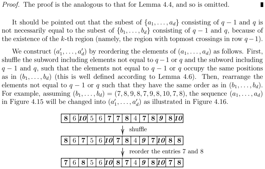
- [§4.2, Lemma 4.6] Lemma 4.6 is load-bearing but its proof is omitted with the words 'the proof is analogous ... and so is omitted.' The statement is not literally analogous to Lemma 4.4: the paper explicitly notes that the multiset of elements equal to q−1 or q need not match between (a_1,...,a_d) and (b_1,...,b_d), precisely because of the k-th region. The subsequent shuffle producing (a′) is well-defined only if Lemma 4.6 holds, and the bijection in Theorem 4.1 depends on that shuffle. A complete proof of this lemma must be supplied before the argument goes through.
- [§4.2, Case 2 (merging step)] The merging step in Section 4.2, Case 2 (Figures 4.15–4.17) is under-specified and inconsistent as displayed. For columns whose F′_j contains q−1 or q, the paper replaces D_j by D_j ∪ [q−2] = [q−2] ∪ {q} and 'correspondingly' replaces C^(1)_j and C′_j by C^(1)_j ∪ [p−2] and C′_j ∪ [p−2]. Three things are missing. First, the equality asserts D_j ⊆ [q−2] ∪ {q}, but the merged columns are selected because their content contains q−1 or q, and [q−2] ∪ {q} contains no q−1; the formula therefore cannot hold as written (it also uses [p−2] where [q−2] appears intended). Second, no proof is given that the modified diagram is normalized and multiplicity-free, satisfies (C1)–(C2), that the modified C-columns still lie below the modified D-columns in Gale order (the sizes of C^(1)_j ∪ [q−2] and [q−2] ∪ {q} do not obviously match), or that the region taxonomy of §3.2 applies to the next iteration of Φ. Third, the iteration in §4.4 and its termination depend on this closure, which is not stated as a lemma. The merging step thus needs to be rewritten as a lemma with explicit hypotheses, construction, and verification.
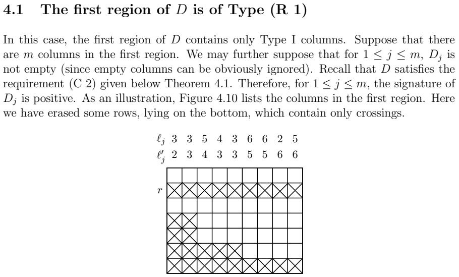
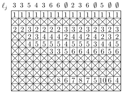
- [§4.3, Type (R3)] The Type (R3) case, one of the three exhaustive region types, is only sketched: the text says the construction is 'nearly the same' as in §4.2 and defines Φ and Φ̂ by reference to the two cases of §4.2. This case differs materially from (R2): p is defined as the second-lowest box of the Type III column D_m rather than as n_m, and the column being adjusted after the first algorithm is the Type III column itself. The analogues of Lemmas 4.5 and 4.6 in this setting are not stated, and the figures do not replace the missing verification that the resulting filling is flagged and has the claimed weight. A full treatment of this case is required for Theorem 4.1 to cover all multiplicity-free diagrams.
- [§3.2 and §4, reductions (C1)–(C2)] The proof of Theorem 4.1 explicitly assumes (C1) (every column has at least two crossings, achieved by embedding into a larger grid) and (C2) (no standard interval column [m]). Of these, (C2) is adequately justified below Lemma 3.3. Reduction (C1), by contrast, is asserted in a single sentence at the beginning of §3.2. Since the entire region taxonomy and the three cases of Φ rest on the presence of a second crossing, the embedding argument should be stated as a lemma: it must show that multiplicity-freeness is preserved by the embedding (checking the twelve configurations), that the embedded diagram has at least two crossings per column, and that the zero-one property of the embedded dual character descends to χ_D. The descent is immediate because the relevant monomials involve only x_1,...,x_n, but the multiplicity-free check is not written down.
minor comments (5)
- [§4.2, after Lemma 4.6] The word 'subest' appears twice in the paragraph following Lemma 4.6; it should be 'subset'.
- [§4.4, sign-preservation argument] In the exchange argument of case (1), the sentence 'Suppose that Fj1 has column reading word u ... and Fj1 has column reading word v' should refer to Fj2 for the second word; as written the notation is inconsistent.
- [§4.4, operation (2)] The claim that reordering row-q entries does not change inversion numbers states that the moved entries are 'bigger' than any entry above; the argument only requires that they are at least as large as every entry above row q in the corresponding column, so that the bottom position of each column reading word never participates in an inversion. The wording should be adjusted, and the fact that the relevant columns have no entries below row q should be stated explicitly.
- [§1, §2, §4.2] There are several typos: 'flagged Weyl models' should be 'flagged Weyl modules' (Introduction), 'northewest diagrams' should be 'northwest diagrams' (Introduction), 'eigensapce' should be 'eigenspace' (Proposition 2.1), and 'frist region' should be 'first region' (§4.2).
- [Theorem 4.1] Theorem 4.1 is stated for normalized multiplicity-free diagrams, but its proof begins by imposing the extra assumptions (C1) and (C2) inside the proof. Stating the reductions as a lemma before the theorem and referencing it from the theorem would make the logical structure of the proof easier to check.
Circularity Check
No significant circularity: the cited determinant expansion from the authors' prior work is an independent computational tool, and the main proof is not definitionally circular.
full rationale
The derivation is self-contained with respect to the claimed criterion. The main reduction, Proposition 2.1, equates zero-oneness with one-dimensional eigenspaces; this is a definitional reformulation of equation (2.1), not a circular use of the target theorem. The converse direction is imported from [23, Proposition 3.11], an external prior result by different authors. The forward proof uses Proposition 2.2, a signed flagged-filling expansion of det(Y_C^D), cited from the authors' own [27]; although this is a self-citation and is load-bearing as a computational tool, the identity is a parameter-free determinant expansion whose assumptions do not include the zero-one criterion, so it qualifies as independent support and does not constitute circularity. The WLOG reductions (C1) and (C2) are explained in the text: embedding into a larger grid supplies the missing crossings, and a standard interval column [m] contributes only the monomial factor x_1...x_m, so neither reduction assumes the conclusion. The proof does contain genuine completeness gaps: Lemma 4.6 is stated with its proof omitted as analogous, and the Type (R3) case in Section 4.3 is only sketched. These are verification gaps, not circular reductions. No equation is used that is definitionally equal to the theorem, and no fitted, renamed, or predicted quantity is presented as an input in disguise.
Assumptions & free parameters
assumptions (4)
- standard math Proposition 2.2: det(Y^C_D) expands as a signed sum over flagged fillings of D, cited from [27, Lemma 2.2].
- standard math Proposition 2.1: χ_D is zero-one if and only if every eigenspace has dimension one.
- standard math χ_D is invariant under reordering the columns of D, so normalization is without loss of generality.
- domain assumption Reductions (C1) and (C2): every column may be assumed to have at least two crossings, and D may be assumed to have no standard interval column [m].
Cite this review
Pith. "Pith review of Zero-one dual characters of flagged Weyl modules." pith.science (2026). https://pith.science/paper/EUM7YBLJ
@misc{pith2026241110933,
  author       = {Pith},
  title        = {Pith review of: Zero-one dual characters of flagged Weyl modules},
  year         = {2026},
  howpublished = {\url{https://pith.science/paper/EUM7YBLJ}},
  note         = {Machine review of arXiv:2411.10933}
}
abstract
We prove a criterion of when the dual character $\chi_{D}(x)$ of the flagged Weyl module associated to a diagram $D$ in the grid $[n]\times [n]$ is zero-one, that is, the coefficients of monomials in $\chi_{D}(x)$ are either 0 or 1. This settles a conjecture proposed by M{\'e}sz{\'a}ros--St. Dizier--Tanjaya. Since Schubert polynomials and key polynomials occur as special cases of dual flagged Weyl characters, our approach provides a new and unified proof of known criteria for zero-one Schubert/key polynomials due to Fink--M{\'e}sz{\'a}ros--St. Dizier and Hodges--Yong, respectively.
Figures


Figures from the paper (21 more)







Forward citations
Cited by 2 Pith papers
-
Schubert polynomials and patterns in permutations
A new lower bound relates the number of supports of Schubert polynomials to weighted counts of twelve permutation patterns, strengthening previous 132 and 1432 bounds.
-
Introduction to the Cohomology of the Flag Variety
A survey chapter presenting the cohomology of flag varieties and Schubert and Schur polynomials as the rigorous basis for solving Schubert's enumerative geometry problems.
Reference graph
Works this paper leans on
-
[23]
M´ esz´ aros, A
K. M´ esz´ aros, A. St. Dizier and A. Tanjaya, Principal specialization of dual characters of flagged Weyl modules, Electron. J. Combin. 28 (2021), Paper No . 4.17, 12 pp
2021
-
[27]
S.C.Y. Peng, Z. Lin and S.C.C. Sun, Upper bounds of dual flagged W eyl characters, Adv. Appl. Math. 160 (2024), 102752, 12pp
work page 2024
- [1]
-
[2]
S. Assaf and D. Searles, Kohnert polynomials, Exp. Math. 31 (1) (2022), 93–119
work page 2022
-
[3]
S. Assaf and D. Searles, Kohnert tableaux and a lifting of quasi-S chur functions, J. Combin. Theory Ser. A 156 (2018), 85–118
work page 2018
-
[4]
F. Castillo, Y. Cid-Ruiz, F. Mohammadi and J. Monta˜ no, K-polyno mials of multiplicity-free varieties, arXiv:2212.13091, 2022
arXiv 2022
-
[5]
M. Brion, Multiplicity-free subvarieties of flag varieties, Commuta tive algebra (Grenoble/Lyon, 2001), Contemp. Math., vol. 331, Amer. Math. S oc., Providence, RI, 2003, pp. 13–23
work page 2001
- [6]
Show all 29 references
-
[7]
Fan and P.L
N.J.Y. Fan and P.L. Guo, Vertices of Schubitopes, J. Combin. Theo ry Ser. A 177 (2021), 105311, 20pp
2021
-
[8]
Fan and P.L
N.J.Y. Fan and P.L. Guo, Upper bounds of schubert polynomials, Sc i. China Math. 65 (2022), 1319–1330
2022
-
[9]
A. Fink, K. M´ esz´ aros and A. St. Dizier, Schubert polynomials as integer point trans- forms of generalized permutahedra, Adv. Math. 332 (2018), 465 –475
2018
-
[10]
A. Fink, K. M´ esz´ aros and A. St. Dizier, Zero-one Schubert p olynomials, Math. Z. 297 (2021), 1023–1042
2021
-
[11]
Y. Gao, R. Hodges and A. Yong, Classification of Levi-spherical Schubert varieties. Selecta Math. (N.S.) 29 (2023), Paper No. 55, 40 pp
2023
-
[12]
Hamaker, O
Z. Hamaker, O. Pechenik and A. Weigandt, Gr¨ obner geometry of Schubert polyno- mials through ice, arXiv:2003.13719, 2020
2003 arXiv
-
[13]
Hodges and A
R. Hodges and A. Yong, Coxeter combinatorics and spherical S chubert geometry, J. Lie Theory 32 (2022), 447–474
2022
-
[14]
Hodges and A
R. Hodges and A. Yong, Multiplicity-free key polynomials, Ann. Co mb. 27 (2023), 387–411
2023
-
[15]
Klein, Diagonal degenerations of matrix Schubert varieties, Algebraic Combin
P. Klein, Diagonal degenerations of matrix Schubert varieties, Algebraic Combin. 6 (2023), 1073–1094
2023
-
[16]
Knutson, T
A. Knutson, T. Lam and D.E. Speyer, Positroid varieties: jugglin g and geometry, Compositio Math. 149 (2013), 1710–1752
2013
-
[17]
Kohnert, Weintrauben, Polynome, Tableaux, Bayreuth Mat h
A. Kohnert, Weintrauben, Polynome, Tableaux, Bayreuth Mat h. Schrift. 38(1990), 1–97
1990
-
[18]
Kraskiewicz and P
W. Kraskiewicz and P. Pragacz, Foncteurs de schubert, C. R. Acad. Sci. Paris S´ er. I Math. 304 (1987), 209–211
1987
-
[19]
Kra´ skiewicz and P
W. Kra´ skiewicz and P. Pragacz, Schubert functors and Schu bert polynomials, Eu- ropean J. Combin. 25 (2004), 1327–1344. 22
2004
-
[20]
Knutson, Frobenius splitting and M¨ obius inversion, arXiv:090 2.1930v1, 2009
A. Knutson, Frobenius splitting and M¨ obius inversion, arXiv:090 2.1930v1, 2009
2009
-
[21]
Knutson and E
A. Knutson and E. Miller, Gr¨ obner geometry of Schubert polyn omials, Ann. Math. 161 (2005), 1245–1318
2005
-
[22]
Magyar, Schubert polynomials and Bott–Samelson varieties, Comment
P. Magyar, Schubert polynomials and Bott–Samelson varieties, Comment. Math. Helv. 73 (1998), 603–636
1998
-
[24]
M´ esz´ aros and A
K. M´ esz´ aros and A. Tanjaya, Inclusion-exclusion on Schubert polynomials, Algebr. Comb. 5 (2022), 209–226
2022
-
[25]
M´ esz´ aros, L
K. M´ esz´ aros, L. Setiabrata and A. St. Dizier, An orthodont ia formula for Grothendieck polynomials, Trans. Amer. Math. Soc. 375 (2022), 1 281–1303
2022
-
[26]
M´ esz´ aros, L
K. M´ esz´ aros, L. Setiabrata and A. St. Dizier, On the suppor t of Grothendieck polynomials, arXiv:2201.09452, 2022
2022 arXiv
-
[28]
Postnikov, Total positivity, Grassmannians, and networks , http://arxiv.org/abs/math/0609764, 2006
A. Postnikov, Total positivity, Grassmannians, and networks , http://arxiv.org/abs/math/0609764, 2006
2006 arXiv
-
[29]
Pechenik and M
O. Pechenik and M. Satriano, Proof of a conjectured M¨ obius in version formula for Grothendieck polynomials, arXiv:2202.02897, 2022. (Peter L. Guo) Center for Combinatorics, Nankai University , LPMC, Tianjin 300071, P.R. China Email address: lguo@nankai.edu.cn (Zhuowei Lin) C...
2022 arXiv
Reviewed August 12, 2026 · model on record in the stance chip above.
Discussion (0). Continue with ORCID to comment.