Mixed-Precision in adaptive Runge-Kutta method for large ODE systems
Pith reviewed 2026-05-25 03:13 UTC · model grok-4.3
The pith
Mixed-precision Runge-Kutta solvers preserve most high-precision accuracy in large ODE systems
A machine-rendered reading of the paper's core claim, the machinery that carries it, and where it could break.
Core claim
Mixed-precision versions of the Bogacki-Shampine 3(2) Runge-Kutta pair preserve most of the accuracy of high-precision solvers under a wide range of tolerances. Accuracy improves with system size to match high-precision performance seen in smaller systems. The arithmetic change does not alter evaluation counts enough to offset the speed benefit of low-precision operations, enabling significant speed-up with little accuracy loss in large coupled ODE systems.
What carries the argument
Mixed-precision Bogacki-Shampine 3(2) Runge-Kutta pair applied to large ODE systems, using low precision for speed and high precision selectively for accuracy control.
If this is right
- Mixed-precision methods can deliver significant computational speed-up for large coupled ODE systems.
- Accuracy remains close to high-precision levels over wide solver tolerances.
- Accuracy performance improves as the ODE system size grows.
- The number of function evaluations is not substantially affected, maintaining the speed benefit.
Where Pith is reading between the lines
- This technique could be tested on other families of ODE solvers such as multistep methods.
- Hardware architectures optimized for low precision might see even larger gains if error control is also adapted.
- The size-dependent accuracy improvement suggests benefits specifically for very large-scale simulations not fully explored in the benchmarks.
Load-bearing premise
The three benchmark systems of coupled oscillators, Kuramoto model, and circadian clock adequately represent large ODE systems containing many heterogeneous interactions.
What would settle it
A demonstration that mixed-precision accuracy drops substantially below high-precision levels for some large ODE system under standard tolerances would challenge the main claim.
Figures



read the original abstract
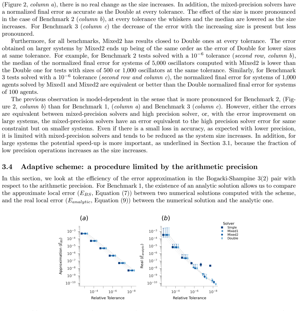
Mixed-precision methods combine low and high precision arithmetics to exploit low precision computational speed and high precision accuracy. Large ODE systems that contain many heterogeneous interactions lead to a high computational cost that could be tackled with mixed-precision solvers. We tested mixedprecision versions of the Bogacki-Shampine 3(2) Runge-Kutta pair over three benchmark systems: coupled linear oscillators, the Kuramoto model and a circadian clock model. Our study is performed in a way that can be adapted to any finite-precision format, software architecture and numerical scheme. We found that mixed-precision solvers can preserve most of the high-precision solver accuracy under a wide range of solver tolerances. Moreover, mixed-precision solver accuracy improves with system size, reaching levels equivalent to high-precision solvers in small system size. We also observed that mixed-precision arithmetic does not impact the number of evaluation in a way that balances the benefit of fast operations in low precision. Taken together, these results show that mixed-precision methods can offer significant computational speed-up at little or no loss of accuracy in large coupled ODE systems.
Editorial analysis
A structured set of objections, weighed in public.
Referee Report
Summary. The manuscript presents an empirical study of mixed-precision arithmetic applied to the adaptive Bogacki-Shampine 3(2) Runge-Kutta method for solving large systems of ODEs. It tests this approach on three benchmark systems—coupled linear oscillators, the Kuramoto model, and a circadian clock model—and reports that mixed-precision solvers maintain most of the accuracy of full high-precision solvers across a range of tolerances, with accuracy improving as system size grows, while not significantly affecting the number of function evaluations, thereby offering computational speed-up at little accuracy loss.
Significance. If the empirical findings prove robust upon detailed verification and generalize beyond the tested models, the work could enable meaningful speed-ups in simulating large coupled ODE systems with minimal accuracy trade-offs, which would be valuable for computational applications in physics, biology, and engineering involving high-dimensional dynamical systems.
major comments (2)
- [Abstract] Abstract: the abstract states empirical findings but supplies no implementation details, error-bar methodology, statistical tests, or description of how mixed-precision arithmetic was realized inside the adaptive step-size controller; claims such as 'accuracy improves with system size' therefore cannot be verified.
- [Numerical experiments] Benchmark systems: the three chosen benchmark systems (coupled oscillators, Kuramoto, circadian clock) have relatively uniform or low-dimensional coupling structures; none is a genuinely large (N ≫ 10^3), stiff, or randomly heterogeneous network. This raises concerns about whether the reported size-dependent accuracy gain is a general property of mixed-precision Runge-Kutta or model-specific.
Simulated Author's Rebuttal
We thank the referee for the constructive report and the recommendation of major revision. We address each major comment below, agreeing to expand the abstract and to add discussion of benchmark limitations while defending the relevance of the chosen systems.
read point-by-point responses
-
Referee: [Abstract] Abstract: the abstract states empirical findings but supplies no implementation details, error-bar methodology, statistical tests, or description of how mixed-precision arithmetic was realized inside the adaptive step-size controller; claims such as 'accuracy improves with system size' therefore cannot be verified.
Authors: We agree the abstract is too concise for full verification. In the revised manuscript we will add a sentence describing the mixed-precision realization (low-precision arithmetic applied only to the function evaluations inside the Bogacki-Shampine pair while retaining high-precision error estimation and step-size control), specify that accuracy is measured by direct comparison of solution trajectories against a reference high-precision run at each tolerance, and note that the size-dependent trend is shown by systematic variation of N in the numerical experiments section rather than by formal statistical tests. revision: yes
-
Referee: [Numerical experiments] Benchmark systems: the three chosen benchmark systems (coupled oscillators, Kuramoto, circadian clock) have relatively uniform or low-dimensional coupling structures; none is a genuinely large (N ≫ 10^3), stiff, or randomly heterogeneous network. This raises concerns about whether the reported size-dependent accuracy gain is a general property of mixed-precision Runge-Kutta or model-specific.
Authors: The three systems were selected because they are standard large-scale coupled ODE benchmarks in the literature and exhibit heterogeneous interactions (phase differences in Kuramoto, multiple regulatory loops in the circadian model). Experiments were performed with system sizes reaching several thousand equations, and the accuracy gain with N is observed consistently. We acknowledge that the models are not stiff or randomly heterogeneous; the revised manuscript will include an explicit limitations paragraph stating that generalization to such networks remains to be verified and suggesting this as future work. revision: partial
Circularity Check
No circularity: purely empirical benchmark study with no derivations or fitted predictions
full rationale
The manuscript reports direct numerical experiments comparing mixed-precision and high-precision Bogacki-Shampine 3(2) integrators on three concrete ODE systems (coupled oscillators, Kuramoto, circadian clock). No equations, ansatzes, uniqueness theorems, or parameter-fitting steps appear in the abstract or described content. Claims about accuracy preservation and size-dependent improvement are presented as observed outcomes of those runs, not as predictions derived from prior fitted quantities or self-citations. The central result therefore does not reduce to its own inputs by construction; the derivation chain is empty and the work is self-contained against external benchmarks.
Axiom & Free-Parameter Ledger
Reference graph
Works this paper leans on
-
[1]
D., Palmer, T., and Smolarkiewicz, P
Ackmann, J., Dueben, P. D., Palmer, T., and Smolarkiewicz, P. K.Mixed-precision for linear solvers in global geophysical flows. Journal of Advances in Modeling Earth Systems 14 , 9 (2022), e2022MS003148. Publisher: Wiley Online Library
work page 2022
-
[2]
Approximation of large-scale dynamical systems: An overview
Antoulas, A. Approximation of large-scale dynamical systems: An overview. IFAC Proceedings Volumes 37, 11 (2004), 19–28
work page 2004
-
[3]
Nonequilibrium dynamical mean-field theory and its applications
Aoki, H., Tsuji, N., Eckstein, M., Kollar, M., Oka, T., and Werner, P. Nonequilibrium dynamical mean-field theory and its applications. Reviews of Modern Physics 86 , 2 (2014), 779–837
work page 2014
-
[4]
Acceler- ating scientific computations with mixed precision algorithms
Baboulin, M., Buttari, A., Dongarra, J., Kurzak, J., Langou, J., Langou, J., Luszczek, P., and Tomov, S. Acceler- ating scientific computations with mixed precision algorithms. Computer Physics Communications 180, 12 (2009), 2526–2533
work page 2009
-
[5]
Baker, J., and Christofides, P. D. Finite-dimensional approximation and control of non-linear parabolic PDE systems. International Journal of Control 73 , 5 (2000), 439–456
work page 2000
-
[6]
Bogacki, P., and Shampine, L. F. A 3 (2) pair of Runge-Kutta formulas. Applied Mathematics Letters 2, 4 (1989), 321–325. Publisher: Elsevier
work page 1989
-
[7]
Bordenave, C., McDonald, D., and Proutiere, A. A particle system in interaction with a rapidly varying environment: Mean field limits and applications. arXiv preprint math/0701363 (2007). 12
work page internal anchor Pith review Pith/arXiv arXiv 2007
-
[8]
Mean-field limits beyond ordinary differential equations
Bortolussi, L., and Gast, N. Mean-field limits beyond ordinary differential equations. Formal Methods for the Quantita- tive Evaluation of Collective Adaptive Systems: 16th International School on Formal Methods for the Design of Computer, Communication, and Software Systems, SFM 2016, Bertinoro, Italy, June 20-24, 2016, Advanced Lectures 16 (2016), 61–82
work page 2016
-
[9]
Brogi, F., Bn`a, S., Boga, G., Amati, G., Ongaro, T. E., and Cerminara, M. On floating point precision in computational fluid dynamics using openfoam. Future Generation Computer Systems 152 (2024), 1–16
work page 2024
-
[10]
Burnett, B., Gottlieb, S., and Grant, Z. J. Stability analysis and performance evaluation of mixed-precision Runge-Kutta methods, Dec. 2022
work page 2022
-
[11]
Butcher, J. C. Numerical methods for ordinary differential equations . John Wiley & Sons, 2016
work page 2016
-
[12]
Cavaglieri, D., and Bewley, T. Low-storage implicit/explicit Runge-Kutta schemes for the simulation of stiff high- dimensional ODE systems. Journal of Computational Physics 286 (2015), 172–193
work page 2015
-
[13]
Rigorous floating- point mixed-precision tuning
Chiang, W.-F., Baranowski, M., Briggs, I., Solovyev, A., Gopalakrishnan, G., and Rakamari ´c, Z. Rigorous floating- point mixed-precision tuning. ACM SIGPLAN Notices 52 , 1 (2017), 300–315
work page 2017
-
[14]
Nvidia A100 GPU: Performance & innovation for GPU computing
Choquette, J., and Gandhi, W. Nvidia A100 GPU: Performance & innovation for GPU computing. In 2020 IEEE Hot Chips 32 Symposium (HCS) (2020), IEEE Computer Society, pp. 1–43
work page 2020
- [15]
-
[16]
Dar, Z., Baiges, J., and Codina, R. Reduced order modeling. In Machine Learning in Modeling and Simulation: Methods and Applications. Springer, 2023, pp. 297–339
work page 2023
-
[17]
Fehlberg, E. Low-order classical Runge-Kutta formulas with stepsize control and their application to some heat transfer problems, vol. 315. National aeronautics and space administration, 1969
work page 1969
-
[18]
Impulses and physiological states in theoretical models of nerve membrane
FitzHugh, R. Impulses and physiological states in theoretical models of nerve membrane. Biophysical journal 1 , 6 (1961), 445–466
work page 1961
-
[19]
Goodwin, B. C. Oscillatory behavior in enzymatic control processes. Advances in enzyme regulation 3 (1965), 425–437
work page 1965
- [20]
-
[21]
Solving Ordinary Differential Equations I: Nonstiff Problems , second revised edition ed., vol
Hairer, E., Norsett, S., and Wanner, G. Solving Ordinary Differential Equations I: Nonstiff Problems , second revised edition ed., vol. 8 of Springer Series in Computational Mathematics . Springer, Jan. 1993
work page 1993
-
[22]
Speeding up and reducing memory usage for scientific machine learning via mixed precision
Hayford, J., Goldman-Wetzler, J., Wang, E., and Lu, L. Speeding up and reducing memory usage for scientific machine learning via mixed precision. Computer Methods in Applied Mechanics and Engineering 428 (2024), 117093
work page 2024
-
[23]
Higham, N. J., and Mary, T. Mixed precision algorithms in numerical linear algebra. Acta Numerica 31 (May 2022), 347–414
work page 2022
-
[24]
Hirsch, M. W., Smale, S., and Devaney, R. L. Differential equations, dynamical systems, and an introduction to chaos . Academic press, 2013
work page 2013
-
[25]
Activations in low precision with high accuracy
Hubrecht, T., Desrentes, O., and de Dinechin, F. Activations in low precision with high accuracy. hal preprint hal- 04776745 (2024)
work page 2024
-
[26]
Ichimura, T., Fujita, K., Yamaguchi, T., Naruse, A., Wells, J. C., Schulthess, T. C., Straatsma, T. P., Zimmer, C. J., Martinasso, M., Nakajima, K., et al. A fast scalable implicit solver for nonlinear time-evolution earthquake city problem on low-ordered unstructured finite elements with artificial intelligence and transprecision computing. In SC18: Inte...
work page 2018
-
[27]
Mixed-precision numerics in scientific applications: survey and perspectives
Kashi, A., Lu, H., Brewer, W., Rogers, D., Matheson, M., Shankar, M., and Wang, F. Mixed-precision numerics in scientific applications: survey and perspectives. arXiv preprint arXiv:2412.19322 (2024)
-
[28]
Kennedy, C. A., Carpenter, M. H., and Lewis, R. M. Low-storage, explicit Runge-Kutta schemes for the compressible Navier-Stokes equations. Applied numerical mathematics 35 , 3 (2000), 177–219
work page 2000
- [29]
-
[30]
Exascale deep learning for climate analytics
Kurth, T., Treichler, S., Romero, J., Mudigonda, M., Luehr, N., Phillips, E., Mahesh, A., Matheson, M., Deslippe, J., Fatica, M., et al. Exascale deep learning for climate analytics. In SC18: International conference for high performance computing, networking, storage and analysis (2018), IEEE, pp. 649–660
work page 2018
-
[31]
Le Grand, S., G ¨otz, A. W., and Walker, R. C. Spfp: Speed without compromise—a mixed precision model for gpu accelerated molecular dynamics simulations. Computer Physics Communications 184 , 2 (2013), 374–380
work page 2013
-
[32]
Lucia, D. J., Beran, P. S., and Silva, W. A. Reduced-order modeling: New approaches for computational physics. Progress in aerospace sciences 40, 1-2 (2004), 51–117
work page 2004
-
[33]
Micikevicius, P., Narang, S., Alben, J., Diamos, G., Elsen, E., Garcia, D., Ginsburg, B., Houston, M., Kuchaiev, O., Venkatesh, G., et al. Mixed precision training. arXiv preprint arXiv:1710.03740 (2017)
work page internal anchor Pith review Pith/arXiv arXiv 2017
-
[34]
Murray, J. D. Mathematical Biology I: An introduction . Springer, 2002
work page 2002
-
[35]
Agent-based modeling of microbial communities
Nagarajan, K., Ni, C., and Lu, T. Agent-based modeling of microbial communities. ACS synthetic biology 11 , 11 (2022), 3564–3574
work page 2022
-
[36]
An active pulse transmission line simulating nerve axon
Nagumo, J., Arimoto, S., and Yoshizawa, S. An active pulse transmission line simulating nerve axon. Proceedings of the IRE 50, 10 (1962), 2061–2070
work page 1962
-
[37]
Palmer, T. N. More reliable forecasts with less precise computations: A fast-track route to cloud-resolved weather and climate simulators? Philosophical Transactions of the Royal Society A: Mathematical, Physical and Engineering Sciences 372 , 2018 (June 2014), 20130391
work page 2018
-
[38]
Paul, T. J., and Kollmannsberger, P. Biological network growth in complex environments: A computational framework. PLOS Computational Biology 16 , 11 (2020), e1008003
work page 2020
-
[39]
E., Khargonekar, P., and Kurdahi, F
Rakka, M., Fouda, M. E., Khargonekar, P., and Kurdahi, F. Mixed-precision neural networks: A survey. arXiv preprint arXiv:2208.06064 (2022). 13
-
[40]
Reduced-precision parametrization: Lessons from an intermediate- complexity atmospheric model
Saffin, L., Hatfield, S., D ¨uben, P., and Palmer, T. Reduced-precision parametrization: Lessons from an intermediate- complexity atmospheric model. Quarterly Journal of the Royal Meteorological Society 146 , 729 (2020), 1590–1607
work page 2020
-
[41]
Shampine, L. F., and Reichelt, M. W. The Matlab ODE suite. SIAM journal on scientific computing 18 , 1 (1997), 1–22. Publisher: SIAM
work page 1997
-
[42]
Strogatz, S. H. Nonlinear dynamics and chaos with student solutions manual: With applications to physics, biology, chemistry, and engineering . CRC press, 2018
work page 2018
-
[43]
BFloat16: the secret to high performance on Cloud TPUs
Wang, S., and Kanwar, P. BFloat16: the secret to high performance on Cloud TPUs. Google Cloud Blog 4 (2019)
work page 2019
-
[44]
IEEE standard for floating-point arithmetic
Zuras, D., Cowlishaw, M., Aiken, A., Applegate, M., Bailey, D., Bass, S., Bhandarkar, D., Bhat, M., Bindel, D., Boldo, S., et al. IEEE standard for floating-point arithmetic. IEEE Std 754 , 2008 (2008), 1–70. 14 A Parameters For all benchmarks we have Tolerances The absolute tolerance is lower or equal than the relative tolerance. Explored parameters All ...
work page 2008
discussion (0)
Sign in with ORCID, Apple, or X to comment. Anyone can read and Pith papers without signing in.