REVIEW 3 major objections 6 minor 51 references
The regularized visible fold revisited
T0 review · 3 major / 6 minor · reviewed 2026-08-14 · deepseek-v4-flash
Pith's one-line read For every sufficiently small $\epsilon>0$, a limit cycle grazing the discontinuity set in the singular limit unfolds into a locally unique saddle-node bifurcation of limit cycles at $\alpha=\epsilon^{2k/(2k+1)}\alpha_2(\epsilon)$, with…
desk verdict A serious blowup analysis that proves the first rigorous version of the grazing saddle-node bifurcation for general regularizations, but the quantitative derivative estimate at the heart of the uniqueness argument is underproved and needs referee scrutiny. read the letter →
The pith
A machine-rendered reading of the paper's core claim, the machinery that carries it, and where it could break.
The reading
What carries the argument
The machinery is the double blowup: first blow up the discontinuity line $y=\epsilon=0$ to a cylinder, then blow up the nonhyperbolic point $T$, the imprint of the visible fold, to a sphere with weights $(2k,k,1)$. In the charts $(\bar r=1)_1$ and $(\bar\epsilon=1)_2$, this desingularizes the fold: the critical manifold ends at a nonhyperbolic saddle $p_a$, while the grazing orbit enters and leaves through hyperbolic points $p_L$ and $p_R$. Partial linearizations near $p_L$ and $p_R$ are combined with a global analysis of the Chini equation $v'=2u+v^{-k}$, the reduced equation for the middle transition map, to obtain the S-shaped derivative profile in Lemmas 3.14 and 3.17. The saddle-node then follows by writing the Poincar\'e map as $Q\circ R^{-1}$ and applying the implicit function theorem in the scaled variables $x=\epsilon^{2k/(2k+1)}x_2$, $\alpha=\epsilon^{2k/(2k+1)}\alpha_2$.
What would settle it
A direct numerical evaluation of the derivative $X'_{C,0}(x_1)$ of the middle transition map, defined through the Chini equation $v'=2u+v^{-k}$, for small $\nu$ and $x_1\in[-1-\zeta,-1+\zeta]$, would settle the key estimate: it must lie strictly between $-1$ and $0$ with negative second derivative; observing any value outside that interval for some small $\nu$ would contradict Lemma 3.14 and with it the uniqueness part of Theorem 1.7.
Extended reading notes
Core claim
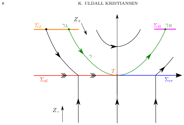
The paper's central claim is Theorem 1.7. Under assumptions (A0)-(A2) on the system and regularization, and (B1)-(B3) on a repelling limit cycle with a single quadratic tangency to the switching manifold, there exists, for all sufficiently small $\epsilon>0$, a locally unique saddle-node bifurcation of limit cycles at $\alpha=\epsilon^{2k/(2k+1)}\alpha_2(\epsilon)$ with $\alpha_2$ continuous. Locally, limit cycles exist precisely for $\alpha\leq\epsilon^{2k/(2k+1)}\alpha_2(\epsilon)$: two for smaller $\alpha$, one at the bifurcation value, and the saddle-node periodic orbit converges in Hausdorff distance to the grazing limit cycle $\Gamma_0$ as $\epsilon\to 0$. This is obtained not from the discontinuous return map but from the regularized transition map itself: Theorem 1.3(d) shows that on an $\epsilon^{2k/(2k+1)}$-neighborhood of the grazing point the map's derivative is monotone, crosses every value in $(-1,0)$ exactly once, and has second derivative uniformly negative, which is exactly the profile needed to separate two fixed points before the bifurcation and none after.
Load-bearing premise
The whole proof hinges on the claimed derivative profile of the middle transition map near the fold—slope strictly between -1 and 0, with decreasing slope—which the paper supports only by a calculation sketch rather than a full proof.
Editorial extensions
If this is right
- For any regularization function satisfying (A1)-(A2), the grazing bifurcation in the regularized system is a genuine saddle-node of limit cycles at the $\epsilon^{2k/(2k+1)}$-scale, where $k$ is the decay rate of the regularization above the fold.
- Below the bifurcation value there are locally exactly two periodic orbits: one attracting whose $\epsilon\to 0$ limit has a sliding segment, and one repelling that converges to the repelling grazing cycle; above the value there are none.
- The saddle-node periodic orbit converges in Hausdorff distance to the grazing limit cycle $\Gamma_0$ as $\epsilon\to 0$, so the bifurcation is a true regularized unfolding of the piecewise-smooth grazing bifurcation.
- In the mass-spring-on-belt example with a Stribeck friction law and a subcritical Hopf bifurcation, the theorem predicts a locally unique saddle-node of limit cycles near the grazing parameter $\alpha_*$ for every small $\epsilon$; the paper's AUTO computation gives a numerically observed slope of about 0.8024, matching the predicted exponent $4/5$ for $k=2$.
- The transition-map description in Theorem 1.3(d) is sharper than previous treatments: in the middle region the map has a single point with any prescribed slope in $(-1,0)$, and the uniform curvature bound rules out additional saddle-nodes.
Reading between the lines
- The transition-map argument is essentially local in the fold, so a natural extension is to higher-dimensional systems whose grazing is a planar quadratic tangency plus strong contraction; one expects the same $\epsilon^{2k/(2k+1)}$ scaling for the saddle-node in that setting.
- If the regularization function is non-monotone and produces a fold in the critical manifold, the same consecutive-blowup framework suggests that the unstable limit cycle can be continued past the tangency to a canard-like bifurcation, a case the paper explicitly leaves open.
- The Chini equation $v'=2u+v^{-k}$ is the scalar model for the middle transition; a computer-assisted or analytic bound on its variational equation could replace the sketched proof of Lemma 3.14 and make the uniqueness proof fully checkable.
- The power law $\alpha_{SN}(\epsilon)-\alpha_* \sim \epsilon^{2k/(2k+1)}$ is a fingerprint of the regularization's decay rate, so measuring the saddle-node shift for different smoothing functions with known $k$ would directly test the theorem's quantitative claim.
Signed reviews
Editorial analysis
A structured set of objections, weighed in public.
Referee Report
Summary. The paper studies singularly perturbed planar systems that limit, as ε→0, to piecewise smooth systems with a visible fold singularity. The main technical result, Theorem 1.3, gives a detailed description of the transition map near the fold under general assumptions (A0)-(A2) on the regularization function, including contraction away from the grazing point, a derivative estimate in an O(ε^{2k/(2k+1)}) neighborhood of the grazing point, and a description of the derivative profile there. Theorem 1.7 then uses this transition map to prove, for a grazing repelling limit cycle satisfying (B1)-(B3), the existence of a locally unique saddle-node bifurcation of limit cycles at α = ε^{2k/(2k+1)} α_2(ε), with exactly two limit cycles below the bifurcation value and one at the value, and with Hausdorff convergence of the saddle-node orbit to the grazing cycle. The proof is built on two consecutive blowups, a partial linearization near the hyperbolic points p_L and p_R, an analysis of a Chini-type equation, and an implicit function argument. Section 2 applies the result to a mass-spring system on a moving belt with a Stribeck friction law and provides AUTO-based numerical evidence, including the predicted exponent 4/5 for k=2.
Significance. If the quantitative estimates in Section 3.5 are supplied in full, the paper would constitute the first rigorous proof of local uniqueness of the saddle-node bifurcation in the regularized grazing bifurcation for the visible fold, extending earlier work by Bonet-Revés and Seara from Sotomayor-Teixeira regularization functions to the class of asymptotic regularization functions satisfying (A1)-(A2). The consecutive-blowup framework is appropriate and general, and the paper gives explicit, falsifiable predictions: the scaling exponent ε^{2k/(2k+1)} in Theorem 1.7 is verified numerically, and the transition-map derivative profile in Theorem 1.3(d) is a concrete quantitative statement. The assumptions (A0)-(A2) and (B1)-(B3) do not appear to encode the conclusion; there is no circular parameter fitting. The application to the Stribeck friction oscillator is a genuine and well-motivated addition. However, the central derivative profile of the middle transition map, Lemma 3.14, is only sketched, and the chain-rule estimate that converts it into the uniform negativity bound in Lemma 3.17 is asserted rather than demonstrated.
major comments (3)
- [Section 3.5, Lemma 3.14 and Lemma 3.17] The proof of Lemma 3.14 is only a sketch, and this is the quantitative core of Theorem 1.3(d)(ii). For the endpoint x1 = -1+ζ the argument invokes 'a simple calculation' together with an odd variational equation to conclude X'_C,0 approaches -1; for x1 = -1-ζ it asserts convergence to 0^- by 'following the flow ... up close to the center manifold of p_a' without any estimate. The uniform negativity of X''_C,0 on the whole interval is inferred from Lemma 3.13, but Lemma 3.13 only gives sign information, not a positive lower bound for |X''_C,0|. These facts are load-bearing: Lemma 3.17 needs X''_ε < -c^{-1} after the rescaling, and Lemma 4.5's nondegeneracy condition (4.7) plus the uniqueness of the saddle-node in Theorem 1.7 depend on that bound. An independent, detailed verification of both endpoint asymptotics and of a uniform bound on X''_C,0 is required.
- [Section 3.5, Lemma 3.16, Eq. (3.47)] The chain-rule estimate in Eq. (3.47) is not justified by the displayed argument. Using the asymptotics (3.44)-(3.45), the contributions to X''_ε coming from the second derivatives of X_R,ε and ~X_L,ε are of order ε^{-2k/(2k+1)} or larger, not O(1); they can be absorbed into the leading term only if those second derivatives are uniformly O(c) and (X_C,ε)'' is bounded away from zero. The proof says 'simple calculation' but does not track these terms. Since Eq. (3.47) is the bridge from Lemma 3.14 to Lemma 3.17 and hence to the nondegeneracy condition (4.7), a complete derivation with all remainders accounted for is needed.
- [Section 3.5, proof of Theorem 1.3(d)(i), and Section 4, Lemma 4.1] The proof of the contraction estimate in Theorem 1.3(d)(i) is only sketched. The first part of the passage from Σ_out,L_L to Σ_in,C_R is described as 'standard and left out of this manuscript completely', and the second part is asserted to be contracting because of exponential contraction toward the center manifold of p_a. This estimate is used in Lemma 4.1 to prove that for α<0 there are exactly two fixed points and for α>0 there are none, which is part of the full statement of Theorem 1.7. Please supply the missing estimates or state and prove the needed contraction bound explicitly.
minor comments (6)
- [Section 3.2, Eqs. (3.19) and (3.23)] In the displayed forms of Ψ_L and Ψ_R, the function ~R_L is written as O(ρ^k_1), but the coordinate change should have the form 1 + O(ρ^k_1) to be invertible near the identity; please clarify the intended expansion.
- [Section 3.2, Eq. (3.26)] There is a typo in the line 'XR(0, 1, 0, ) = 0': an extra comma appears after the third argument.
- [Lemma 3.6] The phrase 'C2 O(ε_1^{1/(2k+1)})-close' is awkward; it should be rephrased as 'C^2 and O(ε_1^{1/(2k+1)})-close' to avoid ambiguity.
- [Section 1.4 and throughout] The paper says it will leave to the reader what 'sufficiently large' smoothness is, but the main theorems rely on C^2 estimates and an implicit function theorem argument. Please state a specific finite order of smoothness for the main results, or at least specify that C^3 or C^4 suffices for Theorem 1.7.
- [Section 2, Figure 5 and surrounding text] The subfigure references are inconsistent: the text refers to 'Fig. 5(d)' for the log-log plot of α*−α, while the caption labels that plot as '(b)', and the caption's '(d)' is the phase portrait. Please align the in-text references with the caption.
- [Section 5, paragraph 'Comparison with previous results'] There is a typo in the phrase '[26, Thoerem 3.3]'; it should read 'Theorem'.
Circularity Check
No significant circularity: the saddle-node result is derived from independent transition-map estimates and standard blowup/Fenichel theory, not encoded in the assumptions.
full rationale
The derivation chain in Theorem 1.7 is not circular. The assumptions (A0)-(A2) and (B1)-(B3) are structural hypotheses about the regularized vector field and the grazing limit cycle; they do not contain the conclusion of a locally unique saddle-node bifurcation. The normal form (1.11) is imported from the external reference [3], not from the author's own prior work. The blowup framework is stated as following [32], which is a self-citation, but the load-bearing analysis is carried out in the manuscript itself: Appendix A gives a proof of Theorem 1.3(a), and Sections 3.2--3.5 derive the transition-map estimates (Lemmas 3.6, 3.8, 3.13-3.17) from direct variational calculations on the blown-up equations and the Chini equation. Lemma 3.13, which supplies U'(u) in (-1,0) and U''(u)<0, is proved in detail. Lemma 3.14 uses this lemma together with stated endpoint asymptotics; those endpoint claims are only sketched ('a simple calculation', 'following the flow ... up close to the center manifold of pa'), but a sketch is a rigor or correctness concern, not circularity, because the claims are not assumed as inputs. The final saddle-node argument applies the implicit function theorem to the fixed-point equation Q2 = R2^{-1}, with nondegeneracy following from the derivative profile and from R's hyperbolic derivative estimates in Lemma 1.6; these ingredients are independent of the advertised uniqueness. The paper also provides an external numerical check (AUTO continuation in Section 2) consistent with the derived scaling. No fitted parameter is renamed as a prediction, and no load-bearing uniqueness theorem is imported from the author's own prior work. Hence the correct circularity finding is no significant circularity, even though the proof of Lemma 3.14 would benefit from a fuller exposition.
Assumptions & free parameters
assumptions (5)
- domain assumption A0-A2: affine dependence in p, smooth monotone asymptotically flat regularization φ, finite algebraic decay rates k± in the tails (1.14)-(1.15).
- domain assumption B1-B3: Z+ has a hyperbolic repelling limit cycle Γ0 tangent to Σ, the tangent point moves across Σ with positive speed in α, and Z− is transverse at the tangency.
- domain assumption Normal form (1.11) from [3, Prop. 14]: a smooth coordinate change puts the visible fold into Z+=(1+f, 2x+yg), Z−=(0,1).
- standard math Fenichel theory, center manifold theory and partial linearization theorems apply as used in Lemmas 3.3-3.9 and Appendix A.
- standard math Implicit function theorem and regular perturbation theory for finite-time flow maps apply to the global return map R and to the Poincaré map P.
Cite this review
Pith. "Pith review of The regularized visible fold revisited." pith.science (2026). https://pith.science/paper/EYHIV4NT
@misc{pith2026190806781,
  author       = {Pith},
  title        = {Pith review of: The regularized visible fold revisited},
  year         = {2026},
  howpublished = {\url{https://pith.science/paper/EYHIV4NT}},
  note         = {Machine review of arXiv:1908.06781}
}
abstract
The planar visible fold is a simple singularity in piecewise smooth systems. In this paper, we consider singularly perturbed systems that limit to this piecewise smooth bifurcation as the singular perturbation parameter $\epsilon\rightarrow 0$. Alternatively, these singularly perturbed systems can be thought of as regularizations of their piecewise counterparts. The main contribution of the paper is to demonstrate the use of consecutive blowup transformations in this setting, allowing us to obtain detailed information about a transition map near the fold under very general assumptions. We apply this information to prove, for the first time, the existence of a locally unique saddle-node bifurcation in the case where a limit cycle, in the singular limit $\epsilon\rightarrow 0$, grazes the discontinuity set. We apply this result to a mass-spring system on a moving belt described by a Stribeck-type friction law.
Figures


Figures from the paper (8 more)


Reference graph
Works this paper leans on
-
[1]
E. J. Berger. Friction modeling for dynamic system simulation. Applied Mechanics Reviews, 55(6):535–577, 2002
work page 2002
-
[2]
C. Bonet and T. M-Seara. Chaos in the hysteretic grazing-sliding codimension-one saddle- node bifurcation of piecewise dynamical systems. In A: Congreso de Ecuaciones Diferenciales y Aplicaciones y Congreso de Matematica Aplicada. ”CEDYA 2017 , pages 73–77, 2017
work page 2017
-
[3]
C. Bonet-Rev´ es and T. M-Seara. Regularization of sliding global bifurcations derived from the local fold singularity of Filippov systems. Discrete and Continuous Dynamical Systems- Series a, 36(7):3545–3601, 2016
work page 2016
-
[4]
E. Bossolini, M. Brøns, and K. U. Kristiansen. Canards in stiction: on solutions of a friction oscillator by regularization. SIAM Journal on Applied Dynamical Systems , 16(4):2233–2258, 2017
work page 2017
-
[5]
E. Bossolini, M. Brøns, and K. U. Kristiansen. Singular limit analysis of a model for earth- quake faulting. Nonlinearity, 30(7):2805–2834, 2017
work page 2017
-
[6]
C. A. Buzzi, P. R. da Silva, and M. A. Teixeira. A singular approach to discontinuous vector fields on the plane. J. Diff. Equations , 231:633–655, 2006
work page 2006
-
[7]
M. Desroches and M. R. Jeffrey. Canards and curvature: nonsmooth approximation by pinch- ing. Nonlinearity, 24(5):1655–1682, May 2011
work page 2011
-
[8]
M. di Bernardo, C. J. Budd, A. R. Champneys, and P. Kowalczyk. Piecewise-smooth Dy- namical Systems: Theory and Applications . Springer Verlag, 2008
work page 2008
Show all 51 references
-
[9]
Dumortier and R
F. Dumortier and R. Roussarie. Canard cycles and center manifolds. Mem. Amer. Math. Soc., 121:1–96, 1996
1996
-
[10]
Ebers and J.L
J.J. Ebers and J.L. Moll. Large-signal behavior of junction transistors. Institute of Radio Engineers – Convention Record, 42(12):1761–1772, 1954
1954
-
[11]
Fenichel
N. Fenichel. Persistence and smoothness of invariant manifolds for flows. Indiana University Mathematics Journal, 21:193–226, 1971
1971
-
[12]
Fenichel
N. Fenichel. Asymptotic stability with rate conditions. Indiana University Mathematics Jour- nal, 23:1109–1137, 1974
1974
-
[13]
Fenichel
N. Fenichel. Geometric singular perturbation theory for ordinary differential equations. J. Diff. Eq., 31:53–98, 1979
1979
-
[14]
Filippov
A.F. Filippov. Differential Equations with Discontinuous Righthand Sides . Mathematics and its Applications. Kluwer Academic Publishers, 1988
1988
-
[15]
Goldbeter and D
A. Goldbeter and D. E. Koshland. An amplified sensitivity arising from covalent modification in biological systems. Proceedings of the National Academy of Sciences , 78(11):6840–6844, 1981
1981
-
[16]
Guglielmi and E
N. Guglielmi and E. Hairer. Classification of hidden dynamics in discontinuous dynamical systems. Siam Journal on Applied Dynamical Systems , 14(3):1454–1477, 2015. 42 K. ULDALL KRISTIANSEN
2015
-
[17]
Heslot, T
F. Heslot, T. Baumberger, B Perrin, B. Caroli, and C. Caroli. Creep, stick-slip, and dry- friction dynamics - experiments and a heuristic model. Physical Review E, 49(6):4973–4988, 1994
1994
-
[18]
S. J. Hogan, M. E. Homer, M. R. Jeffrey, and R. Szalai. Piecewise smooth dynamical systems theory: The case of the missing boundary equilibrium bifurcations. Journal of Nonlinear Science, 26(5):1161–1173, 2016
2016
-
[19]
Jelbart, K
S. Jelbart, K. U. Kristiansen, P. Szmolyan, and M. Wechselberger. Singularly perturbed oscillators with exponential nonlinearities. 2019
2019
-
[20]
Jelbart, K
S. Jelbart, K. U. Kristiansen, and M. Wechselberger. Singularly perturbed boundary-focus bifurcations. arXiv preprint 2006.06087 , 2020
2006 arXiv
-
[21]
C.K.R.T. Jones. Geometric Singular Perturbation Theory, Lecture Notes in Mathematics, Dynamical Systems (Montecatini Terme). Springer, Berlin, 1995
1995
-
[22]
Kaklamanos and K
P. Kaklamanos and K. U. Kristiansen. Regularization and geometry of piecewise smooth systems with intersecting discontinuity sets. Siam Journal on Applied Dynamical Systems , 18(3):1225–1264, 2019
2019
-
[23]
Kosiuk and P
I. Kosiuk and P. Szmolyan. Geometric singular perturbation analysis of an autocatalator model. Discrete and Continuous Dynamical Systems - Series S , 2(4):783–806, 2009
2009
-
[24]
Kosiuk and P
I. Kosiuk and P. Szmolyan. Scaling in singular perturbation problems: Blowing up a relaxation oscillator. Siam Journal on Applied Dynamical Systems, Siam J. Appl. Dyn. Syst, Siam J a Dy, Siam J Appl Dyn Syst, Siam Stud Appl Math , 10(4):1307–1343, 2011
2011
-
[25]
Kosiuk and P
I. Kosiuk and P. Szmolyan. Geometric analysis of the Goldbeter minimal model for the embryonic cell cycle. Journal of Mathematical Biology, J. Math. Biol, J Math Biol , 2015
2015
-
[26]
K. U. Kristiansen. Blowup for flat slow manifolds. Nonlinearity, 30(5):2138–2184, 2017
2017
-
[27]
K. U. Kristiansen. A new type of relaxation oscillation in a model with rate-and- state friction. arXiv:1903.12232 e-prints, submitted for publication in Nonlinearity , 2019. https://arxiv.org/pdf/1903.12232.pdf
1903 arXiv
-
[28]
K. U. Kristiansen. Geometric singular perturbation analysis of a dynamical target mediated drug disposition model. Journal of Mathematical Biology , 79(1):187–222, 2019
2019
-
[29]
K. U. Kristiansen and P. Szmolyan. Relaxation oscillations in substrate-depletion oscillators close to the nonsmooth limit. arXiv:1909.11746 e-prints , 2019. https://arxiv.org/pdf/1909.11746.pdf
1909 arXiv
-
[30]
Uldall Kristiansen and S
K. Uldall Kristiansen and S. J. Hogan. On the use of blowup to study regularizations of singu- larities of piecewise smooth dynamical systems in R3. SIAM Journal on Applied Dynamical Systems, 14(1):382–422, 2015
2015
-
[31]
Uldall Kristiansen and S
K. Uldall Kristiansen and S. J. Hogan. Regularizations of two-fold bifurcations in planar piecewise smooth systems using blowup. SIAM Journal on Applied Dynamical Systems , 14(4):1731–1786, 2015
2015
-
[32]
Uldall Kristiansen and S
K. Uldall Kristiansen and S. J. Hogan. Resolution of the piecewise smooth visible-invisible two-fold singularity in R3 using regularization and blowup. Journal of Nonlinear Science , 29(2):723–787, 2018
2018
-
[33]
Krupa and P
M. Krupa and P. Szmolyan. Extending geometric singular perturbation theory to nonhyper- bolic points - fold and canard points in two dimensions. SIAM Journal on Mathematical Analysis, 33(2):286–314, 2001
2001
-
[34]
Krupa and P
M. Krupa and P. Szmolyan. Relaxation oscillation and canard explosion. Journal of Differ- ential Equations, 174(2):312–368, 2001
2001
-
[35]
C. Kuehn. Multiple Time Scale Dynamics . Springer-Verlag, Berlin, 2015
2015
-
[36]
Yu. A. Kuznetsov, S. Rinaldi, and A. Gragnani. One parameter bifurcations in planar Filippov systems. Int. J. Bif. Chaos , 13:2157–2188, 2003
2003
-
[37]
K. J. Laidler. Chemical kinetics. Harper & Row, 1987
1987
-
[38]
Llibre, P
J. Llibre, P. R. da Silva, and M. A. Teixeira. Regularization of discontinuous vector fields on R3 via singular perturbation. J. Dyn. Diff. Eq. , 19:309–331, 2007
2007
-
[39]
Llibre, P
J. Llibre, P. R. Da Silva, and M. A. Teixeira. Study of singularities in nonsmooth dynamical systems via singular perturbation. Siam Journal on Applied Dynamical Systems , 8(1):508– 526, 2009
2009
-
[40]
Makarenkov and J
O. Makarenkov and J. S. W. Lamb. Dynamics and bifurcation of nonsmooth systems: A survey. Physica D, 241:1826–1844, 2012
2012
-
[41]
J. R. Munkres. Topology. Pearson,, 2000. THE REGULARIZED VISIBLE FOLD REVISITED 43
2000
-
[42]
F. W. J. Olver, D. W. Lozier, R. F. Boisvert, and C. W. Clark. Nist handbook of mathematical functions. Journal of Geometry and Symmetry in Physics , pages 99–104, 2011
2011
-
[43]
Panazzolo and P
D. Panazzolo and P. R. da Silva. Regularization of discontinuous foliations: Blowing up and sliding conditions via fenichel theory. Journal of Differential Equations , 263(12):8362–8390, 2017
2017
-
[44]
Papangelo, M
A. Papangelo, M. Ciavarella, and N. Hoffmann. Subcritical bifurcation in a self-excited single- degree-of-freedom system with velocity weakeningstrengthening friction law: analytical re- sults and comparison with experiments. Nonlinear Dynamics, 90(3):2037–2046, 2017
2017
-
[45]
L. Perko. Differential equations and dynamical systems . Springer,, 2001
2001
-
[46]
Schecter
S. Schecter. Exchange lemmas 2: General exchange lemma. Journal of Differential Equations, 245(2):411–441, 2008
2008
-
[47]
Sotomayor and M
J. Sotomayor and M. A. Teixeira. Regularization of discontinuous vector fields. InProceedings of the International Conference on Differential Equations, Lisboa , pages 207–223, 1996
1996
-
[48]
Szmolyan
P. Szmolyan. Progress and challenges in singular perturbations. Talk at EquaDiff Conference in Bratislava, Slovakia, July 2017
2017
-
[49]
J. J. Tyson, K. C. Chen, and B. Novak. Sniffers, buzzers, toggles and blinkers: Dynamics of regulatory and signaling pathways in the cell. Current Opinion in Cell Biology , 15(2):221– 231, 2003
2003
-
[50]
V.I. Utkin. Sliding Modes in Control and Optimization . Springer, 1992
1992
-
[51]
H. I. Won and J. Chung. Stickslip vibration of an oscillator with damping. Nonlinear Dy- namics, 86(1):257–267, 2016
2016
Reviewed August 14, 2026 · model on record in the stance chip above.
Discussion (0). Continue with ORCID to comment.