REVIEW 2 major objections 5 minor 1 cited by
Numerical inverse scattering transform for the defocusing nonlinear Schr\"odinger equation with box-type initial conditions on a nonzero background
T0 review · 2 major / 5 minor · reviewed 2026-08-10 · deepseek-v4-flash
Pith's one-line read The paper presents a numerical inverse scattering transform for the defocusing NLS equation with box-type initial conditions on a nonzero background, and demonstrates accuracy in both asymptotic regions of the (x,t)-plane.
desk verdict Serious numerical IST paper for NLS on nonzero background with discontinuous box data; the main caveat is an openly admitted unproven existence statement for the deformed RHP, which should be fixed or clearly flagged as a conjecture. read the letter →
The pith
A machine-rendered reading of the paper's core claim, the machinery that carries it, and where it could break.
The reading
What carries the argument
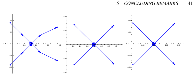
The load-bearing object is the deformed Riemann–Hilbert problem RHP 5 for the transformed unknown $\tilde m(z)$ in the solitonic region and its analogue in the solitonless region. RHP 5 is obtained after three moves: opening lenses along rays where the oscillatory exponentials $\exp(\pm 2ti\Theta(\xi,z))$ decay; solving a scalar Riemann–Hilbert problem for $\delta(z)$ that absorbs the jump on part of the real axis; and multiplying by $E(z)=I_2 + q_o \sigma_2 e^{-i\theta\sigma_3} z^{-1} \tilde m(0)^{-1}$ to remove the $1/z$ singularity at $z=0$. The payoff is a regular Riemann–Hilbert problem with determinant one, whose jump matrices are exponentially close to the identity for large $t$, so Chebyshev collocation converges rapidly and the computational cost is essentially independent of $x$ and $t$.
What would settle it
Evaluate the Wronskian $W(\hat m_2(q_o),\hat m_1(-q_o))$ from Eq. (167) on a fine grid of $(x,t)$ with $t>0$ for the box parameters (59); a single zero would mean RHP 5 has no solution there and the reconstructed $q(x,t)$ cannot be trusted. A sharper version is to test $\theta=\pi/2$, where the paper itself shows the solvability condition fails at $t=0$, and look for failure at small $t>0$.
Extended reading notes
Core claim
The central discovery is that the inverse scattering transform for the defocusing NLS equation on a nonzero background can be made fully numerical even when the initial data are discontinuous and do not decay at infinity, provided the scattering data are known explicitly and no solitons are present. Working in the uniformization variable $z=k+\lambda$, $\lambda=\sqrt{k^2-q_o^2}$, removes the square-root branching of the spectral problem. The paper then applies a sequence of lens-opening deformations, a scalar Riemann–Hilbert problem for a function $\delta$ that removes the jump on part of the real axis, and a final transformation $E(z)$ that removes the remaining singularity at $z=0$; the resulting regular Riemann–Hilbert problem for the unknown $\tilde m$ is solved by Chebyshev collocation. Reconstructing $q(x,t)$ from the large-$z$ behavior of $\tilde m$ yields the solution at any $(x,t)$. The method is verified by residual checks against the NLS equation, by Cauchy-error convergence in the collocation degree, and by comparison with a heavily damped Fourier method; the presented runs reach a residual of $2.5\times 10^{-5}$ at $(x,t)=(-11,5)$ and show the claimed seconds-scale cost.
Load-bearing premise
The load-bearing premise is that the deformed Riemann–Hilbert problem for the final unknown $\tilde m$ has a solution for every $t>0$ in the tested regions; the paper proves this only at $t=0$ and otherwise checks the solvability condition numerically after the fact.
Editorial extensions
If this is right
- For any box initial condition free of discrete spectrum, the solution $q(x,t)$ can be evaluated at a single point in seconds, with accuracy that improves as $t$ grows because the deformed jumps decay exponentially.
- The approach removes the need to resolve the nonlinear Gibbs phenomenon: discontinuous initial data are handled directly, whereas a Fourier method required a period of length 800 and over a million modes to reach $10^{-3}$ accuracy at $t=1$.
- The solvability condition $W(\hat m_2(q_o),\hat m_1(-q_o))\neq 0$ can be checked after each computation, giving a built-in test of whether the reconstructed $q(x,t)$ is trustworthy at that $(x,t)$.
- The same deformed-RHP construction works in both asymptotic regions $|x/(2t)|<q_o$ and $|x/(2t)|>q_o$, and the numerical solutions from the two regions agree across the collisionless-shock boundary for bounded times.
Reading between the lines
- If RHP 5 is later proved to have a solution for all $t>0$ (currently open), the method would become a fully rigorous numerical IST for this class of data; until then, a zero of the solvability Wronskian would mark a genuine boundary of the method's validity.
- The same contour-deformation and singularity-removal machinery should extend to initial data with a few solitons, by converting residue conditions into jumps, and to smooth non-decaying data, at the cost of adding a $\bar\partial$-problem for the reflection coefficient.
- Because evaluation cost is independent of $x$ and $t$, the method is well suited to generating tables of "nonlinear special functions" for the defocusing NLS, analogous to the role numerical Riemann–Hilbert solvers play for Painlevé transcendents.
- A direct test of the open existence question would be to run the solver for phases near $\theta=\pi/2$, where the paper shows the solvability condition already fails at $t=0$, and see whether failures persist at small $t>0$.
Signed reviews
Editorial analysis
A structured set of objections, weighed in public.
Referee Report
Summary. This manuscript presents a numerical inverse scattering transform (IST) for the defocusing nonlinear Schrödinger equation with constant nonzero boundary conditions and a box-type initial condition, in the solitonless case. The scattering data are obtained in closed form through the uniformization variable z, and the inverse problem is reformulated as a sequence of Riemann--Hilbert problems deformed à la Deift--Zhou, with the singularity at z=0 removed by an auxiliary problem, RHP 5 for e_m. The final RHPs are solved by Chebyshev collocation using the authors' RHPackage and ISTPackage, and the method is tested by a finite-difference PDE residual, a damped Fourier spectral comparison, and a Cauchy error study. The central claims are that the method is accurate in both asymptotic regions |x/(2t)|<q_o and |x/(2t)|>q_o, and that evaluating q(x,t) costs effectively independent of x and t.
Significance. The paper attacks a genuinely new case for numerical IST: the defocusing NLS equation with a discontinuous, non-decaying initial condition. If the method is reliable, it goes substantially beyond prior work on Schwartz-class data and provides a practical tool for large-time asymptotics where direct time-stepping is prohibitive. The analytic development is detailed and mostly careful: explicit scattering coefficients, deformation contours with sign charts, analytic treatment of the logarithmic singularity in the delta function, and a clearly stated set of lemmas and propositions. The paper also honestly discloses its main limitation, the open existence question for RHP 5, rather than hiding it. These strengths make the manuscript a plausible important contribution, but the unresolved existence question and the narrow quantitative validation prevent acceptance in the present form.
major comments (2)
- [Section 3.3.1, RHP 5, Remarks 12--13, Eq. (167)] Existence of a solution to the deformed RHP 5 is stated to be open, and the a posteriori solvability condition (167) is the only safeguard. The Chebyshev collocation discretization always yields a finite-dimensional linear system, so a numerically computed e_m can exist even when the true RHP 5 has no solution; checking (167) after the fact is not guaranteed to detect this. Because the reconstruction (93)--(100) uses this e_m, the advertised validity for all (x,t) in the two asymptotic regions rests on an unproved analytic fact. I ask the authors either to prove existence in the parameter regimes under consideration, or to state the main claim conditionally, or to provide a decisive numerical probe such as a dense sweep of the Wronskian (167) over the (x,t) plane in both regions, which would make silent failure implausible.
- [Section 4, Fig. 18, finite-difference residual] The only quantitative convergence and residual tests are performed in the solitonless regime: the Cauchy error is computed at x=-400, t=100 (so xi=-2), and the PDE residual is reported at x=-11, t=5 (so xi=-1.1). No equivalent error study is presented in the solitonic region |x/(2t)|<1, where the contour deformations and the removal of the singularity at z=0 are the most delicate. The abstract's phrase "demonstrated to be accurate within the two asymptotic regions" is therefore stronger than the numerical evidence supports; at least one quantitative convergence test for a point in the solitonic region is needed.
minor comments (5)
- [Remark 17, Appendix D] Remark 17 appears self-contradictory: it states that the solvability condition (167) is satisfied at t=0 if and only if theta=+-pi/2, but then displays the unique e_m(0) for theta different from +-pi/2; the first clause should presumably read "if and only if theta is different from +-pi/2."
- [Eq. (100)] Equation (100) uses e_m^(-1)(x,t) without defining it; specify that this is the coefficient of 1/z in the expansion e_m(z)=I + e_m^(-1)/z + O(z^(-2)).
- [Section 1, runtime claim] The claim that evaluating the solution is "a matter of seconds" is not supported by timing data or a hardware description; a brief timing statement would make the computational advantage reproducible.
- [Data availability] The code is described as "will be made available" as electronic supplementary material; for reproducibility, include the archival link or DOI in the manuscript.
- [Figure 18] The caption and surrounding text do not state explicitly which asymptotic regime the Cauchy-error point x=-400, t=100 belongs to; state xi=-2 so the reader can immediately see that this test is in the solitonless region.
Circularity Check
No significant circularity; the numerical IST derivation is self-contained and validated against the PDE residual and an independent Fourier solver.
full rationale
The central claim is that a deformed-RHP solver computes q(x,t) for solitonless box initial conditions. No parameter is fitted to the target solution: the box parameters (59) are fixed a priori, the reflection coefficient is computed explicitly from (29)/(60), and q(x,t) is reconstructed from the RHP solution via (100). The accuracy statements are supported by (i) substituting the computed q into the NLS equation with a second-order finite-difference residual (Section 4, error 0.000025 at x=-11, t=5), (ii) comparison with a damped Fourier spectral method with over a million modes, and (iii) Cauchy-error convergence |q(x,t,n)-q(x,t,100)| (Fig. 18). These are external or internal consistency benchmarks, not built-in equivalences. The cited no-discrete-spectrum conditions from [5] (shared author) are independent proven constraints on the box parameters, and the paper also states that for (59) a(z) has no zeros in C+; likewise [14] supplies independent scattering asymptotics. The software packages [26,31] are tools, not circular evidence. The paper explicitly flags the open existence question for RHP 5 (Remark 12: 'The question of existence of solution of RHP 5 remains an open problem'; Remark 13: a proof for t>0 'is currently not available') and the a-posteriori solvability check (167); this is a correctness/validity limitation of the arbitrary-(x,t) claim, not a circular reduction, because the numerical scheme is not defined in terms of the quantity it predicts. No equation in the paper reduces by construction to its input.
Assumptions & free parameters
free parameters (2)
- Box IC parameters (q_o, h, L, theta, alpha) =
q_o=1, h=1.5, L=1, theta=0, alpha=0; also theta=0.15 in one example
- Cauchy integral truncation limits =
s in [-10^3,-10^-3] union [10^-3,10^3]
assumptions (3)
- domain assumption The IST scattering theory (Jost eigenfunctions, scattering data, RHP formulation) remains valid for the discontinuous box-type IC despite the IC lying outside the H^{1,1}+tilde-q functional class.
- domain assumption The reflection coefficient rho(z) for the box IC is analytic in the entire complex plane, so no dbar problem arises during contour deformations.
- standard math Standard RHP theory (Plemelj formulas, Liouville theorem, Olver's collocation framework) applies to the deformed RHPs on the chosen contours.
Cite this review
Pith. "Pith review of Numerical inverse scattering transform for the defocusing nonlinear Schr\"odinger equation with box-type initial conditions on a nonzero background." pith.science (2026). https://pith.science/paper/F23PY3B6
@misc{pith2026241219703,
  author       = {Pith},
  title        = {Pith review of: Numerical inverse scattering transform for the defocusing nonlinear Schr\"odinger equation with box-type initial conditions on a nonzero background},
  year         = {2026},
  howpublished = {\url{https://pith.science/paper/F23PY3B6}},
  note         = {Machine review of arXiv:2412.19703}
}
abstract
We present a method to solve numerically the Cauchy problem for the defocusing nonlinear Schr\"{o}dinger (NLS) equation with a box-type initial condition (IC) having a nontrivial background of amplitude $q_o>0$ as $x\to \pm \infty$ by implementing numerically the corresponding Inverse Scattering Transform (IST). The Riemann--Hilbert problem associated to the inverse transform is solved numerically by means of appropriate contour deformations in the complex plane following the numerical implementation of the Deift-Zhou nonlinear steepest descent method. In this work, the box parameters are chosen so that there is no discrete spectrum (i.e., no solitons). The numerical method is demonstrated to be accurate within the two asymptotic regimes corresponding to two different regions of the $(x,t)$-plane depending on whether $|x/(2t)| < q_o$ or $|x/(2t)| > q_o$, as $t \to \infty$.
Figures


Figures from the paper (15 more)




Forward citations
Cited by 1 Pith paper
-
Large-time asymptotics for the defocusing Manakov system on a nonzero background
The defocusing Manakov system on a nonzero background has long-time soliton-region asymptotics given by a modulated N-soliton plus an explicit t^{-1/2} radiation correction.
Reference graph
Works this paper leans on
-
[1]
ARobustInverseScatteringTransformfortheFocusingNonlinearSchrödingerEquation
D.BilmanandP.Miller,“ARobustInverseScatteringTransformfortheFocusingNonlinearSchrödingerEquation”.Comm. Pure App. Math. LXXII, 1722–1805 (2019)
work page 2019
-
[2]
Computation of large-genus solutions of the Korteweg–de Vries equation
D. Bilman, P. Nabelek, and T. Trogdon (2023).“Computation of large-genus solutions of the Korteweg–de Vries equation”. Physica D: Nonlinear Phenomena,449, 133715 (2023)
work page 2023
-
[3]
OnnumericalinversescatteringfortheKorteweg-deVriesequationwithdiscontinuousstep-like data
D.BilmanandT.Trogdon,“OnnumericalinversescatteringfortheKorteweg-deVriesequationwithdiscontinuousstep-like data”, Nonlinearity,33(5), 2211–2269 (2020)
work page 2020
-
[4]
Numerical Inverse Scattering for the Toda lattice
D. Bilman and T. Trogdon,“Numerical Inverse Scattering for the Toda lattice”. Comm. Math. Phys.352, 805–879 (2017)
work page 2017
-
[5]
G.BiondiniandB.Prinari,“OnthespectrumoftheDiracoperatorandtheexistenceofdiscreteeigenvaluesforthedefocusing nonlinear Schr¨dinger equation”. Stud. App. Math.132(2), 138–159 (2014)
work page 2014
-
[6]
On the asymptotic stability of𝑁-soliton solutions of the defocusing nonlinear Schr¨dinger equation
S. Cuccagna and R. Jenkins,“On the asymptotic stability of𝑁-soliton solutions of the defocusing nonlinear Schr¨dinger equation”. Comm. Math. Phys.343(3), 921–969 (2016)
work page 2016
-
[7]
Long-time asymptotics for integrable nonlinear wave equations
P. Deift, A. Its and X. Zhou,“Long-time asymptotics for integrable nonlinear wave equations”. Important Developments in Soliton Theory, Springer Ser. Nonlin. Dyn., pp. 181–204 (Springer, Berlin 1993)
work page 1993
-
[8]
P. Deift, S. Venakides and X. Zhou,“New results in small dispersion KdV by an extension of the steepest descent method for Riemann-Hilbert problems”. IMRN: International Mathematics Research Notices, 1997.6 (1997)
work page 1997
Show all 39 references
-
[9]
A steepest descent method for oscillatory Riemann-Hilbert problems. Asymptotics for the MKdV equation
P. Deift and X. Zhou,“A steepest descent method for oscillatory Riemann-Hilbert problems. Asymptotics for the MKdV equation”. Ann. Math,137295–368, 1993
1993
-
[10]
Long-time asymptotics for integrable systems. Higher order theory
P. Deift and X. Zhou,“Long-time asymptotics for integrable systems. Higher order theory”. Comment. Phys. Math.165, 175–191 (1994)
1994
-
[11]
Long-TimeBehavioroftheNon-FocusingNonlinearSchrödingerEquation,aCaseStudy
P.DeiftandX.Zhou,“Long-TimeBehavioroftheNon-FocusingNonlinearSchrödingerEquation,aCaseStudy”.Lectures in Mathematical Sciences, New Ser., vol. 5, Graduate School of Mathematical Sciences, University of Tokyo, p. 61 (1994)
1994
-
[12]
Long-time asymptotics for solutions of the NLS equation with initial data in a weighted Sobolev space
P. Deift and X. Zhou,“Long-time asymptotics for solutions of the NLS equation with initial data in a weighted Sobolev space”. Commun. Pure Appl. Math.56, 1029–1077 (2003)
2003
-
[13]
An extension of the steepest descent method for Riemann–Hilbert problems: the small dispersion limit of the Korteweg–de Vries equation
P. Deift, X. Zhou and S. Venakides,“An extension of the steepest descent method for Riemann–Hilbert problems: the small dispersion limit of the Korteweg–de Vries equation”. Proc. Natl. Acad. Sci.95(2), 445–454 (1998)
1998
-
[14]
The inverse scattering transform for the defocusing nonlinear Schrödinger equation with nonzero boundary conditions
F. Demontis, B. Prinari, C. van der Mee and F. Vitale,“The inverse scattering transform for the defocusing nonlinear Schrödinger equation with nonzero boundary conditions”. Stud. App. Math.131, 1–40 (2013)
2013
-
[15]
Long-timeasymptoticsfortheNLSequationviadbarmethods
M.Dieng,andK.McLaughlin,“Long-timeasymptoticsfortheNLSequationviadbarmethods”.arXiv:0805.2807(2008)
2008 arXiv
-
[16]
A nonlinear Gibbs-type phenomenon for the defocusing nonlinear Schro¨dinger equation
J.C. DiFranco and K.T.-R. McLaughlin,“A nonlinear Gibbs-type phenomenon for the defocusing nonlinear Schro¨dinger equation”. IMRP Int. Math. Res. Pap.2005, pp. 403–549 (2005)
2005
-
[17]
L. D. Faddeev and L. A. Takhtajan, Hamiltonian methods in the theory of solitons (Springer, Berlin, 1987)
1987
-
[18]
A numerical implementation of Fokas boundary integral approach: Laplace’s equation on a polygonal domain
B. Fornberg and N. Flyer,“A numerical implementation of Fokas boundary integral approach: Laplace’s equation on a polygonal domain”. Royal Society Proc Series A467, 2983–3003 (2011)
2011
-
[19]
Schrödinger group on Zhidkov spaces
C. Gallo,“Schrödinger group on Zhidkov spaces”. Adv. Diff. Eqs.9, 509–538 (2004)
2004
-
[20]
TheCauchyproblemfordefocusingnonlinearSchrödingerequationswithnon-vanishinginitialdataatinfinity
C.Gallo,“TheCauchyproblemfordefocusingnonlinearSchrödingerequationswithnon-vanishinginitialdataatinfinity”. Commun. Partial Differ. Equ.33, 729–771 (2008)
2008
-
[21]
Fourth-order time-stepping for stiff PDEs
A.-K. Kassam and L.N. Trefethen,“Fourth-order time-stepping for stiff PDEs”. SIAM J. Sci. Comput.26, 1214–1233 (2005)
2005
-
[22]
Fourthordertime-steppingforlowdispersionKorteweg-deVriesandnonlinearSchrödingerequations
C.Klein,“Fourthordertime-steppingforlowdispersionKorteweg-deVriesandnonlinearSchrödingerequations”.Electron. Trans. Numer. Anal.29, 116–135 (2008)
2008
-
[23]
Anartificially-dampedFouriermethodfordispersiveevolutionequations
A.LiuandT.Trogdon,“Anartificially-dampedFouriermethodfordispersiveevolutionequations”. App.Num.Math.192, 19–40 (2023). D ON THE DETERMINANT, SYMMETRIES AND SINGULARITIES OFe𝑚55
2023
-
[24]
The ¯𝜕steepestdescentmethodandtheasymptoticbehaviorofpolynomialsorthogonal ontheunitcirclewithfixedandexponentiallyvaryingnonanalyticweights
K.T.-R.McLaughlinandP.D.Miller,“The ¯𝜕steepestdescentmethodandtheasymptoticbehaviorofpolynomialsorthogonal ontheunitcirclewithfixedandexponentiallyvaryingnonanalyticweights”.IMRPInt.Math.Res.Pap.(2006),Art.ID48673, 1–77 (2006)
2006
-
[25]
The ¯𝜕steepest descent method for orthogonal polynomials on the real line with varying weights
K.T.-R. McLaughlin and P.D. Miller,“The ¯𝜕steepest descent method for orthogonal polynomials on the real line with varying weights”. Int. Math. Res. Not. IMRN, Art. ID rnn 075, 66 pp (2008)
2008
-
[26]
Olver, RHPackage, https://github.com/dlfivefifty/RHPackage (2010)
S. Olver, RHPackage, https://github.com/dlfivefifty/RHPackage (2010)
2010
-
[27]
A general framework for solving Riemann–Hilbert problems numerically
S. Olver,“A general framework for solving Riemann–Hilbert problems numerically”. Numer. Math.122, 305–340 (2012)
2012
-
[28]
Fast algorithms using orthogonal polynomials
S. Olver, R.M. Slevinsky and A. Townsend,“Fast algorithms using orthogonal polynomials”. Acta Numerica29, 573–699 (2020)
2020
-
[29]
Nonlinear steepest descent and the numerical solution of Riemann–Hilbert problems
S. Olver and T. Trogdon,“Nonlinear steepest descent and the numerical solution of Riemann–Hilbert problems”. Comm. Pure Appl. Math.67, 1353–1389 (2014)
2014
-
[30]
InversescatteringtransformforthevectornonlinearSchrödingerequationwith non-vanishing boundary conditions
B.Prinari,M.J.AblowitzandG.Biondini,“InversescatteringtransformforthevectornonlinearSchrödingerequationwith non-vanishing boundary conditions”, J. Math. Phys.47, 063508, 33pp (2006)
2006
-
[31]
Trogdon, ISTPackage, https://bitbucket.org/trogdon/istpackage (2013)
T. Trogdon, ISTPackage, https://bitbucket.org/trogdon/istpackage (2013)
2013
-
[32]
Numerical inverse scattering for the focusing and defocusing nonlinear Schrödinger equations
T. Trogdon and S. Olver,“Numerical inverse scattering for the focusing and defocusing nonlinear Schrödinger equations”. Proc. Roy. Soc. Lon. A469, 20120330 (2013)
2013
-
[33]
T.TrogdonandS.Olver,Riemann–HilbertProblems,TheirNumericalSolution,andtheComputationofNonlinearSpecial Functions (SIAM, Philadelphia, 2015)
2015
-
[34]
NumericalinversescatteringfortheKorteweg–deVriesandmodifiedKorteweg–de Vries equations
T.Trogdon,S.OlverandB.Deconinck,“NumericalinversescatteringfortheKorteweg–deVriesandmodifiedKorteweg–de Vries equations”. Physica D241, 1003–1025 (2012)
2012
-
[35]
Long-time asymptotics of solutions to the Cauchy problem for the defocusing nonlinear Schrödinger equation with finite-density initial data. I. Solitonless sector
A.H. Vartanian,“Long-time asymptotics of solutions to the Cauchy problem for the defocusing nonlinear Schrödinger equation with finite-density initial data. I. Solitonless sector”. In: Recent developments in integrable systems and Rie- mann–Hilbert problems (Birmingham, AL, 20...
2003
-
[36]
Long-time asymptotics of solutions to the Cauchy problem for the defocusing nonlinear Schrödinger equation with finite-density initial data. II. Dark solitons on continua
A.H. Vartanian,“Long-time asymptotics of solutions to the Cauchy problem for the defocusing nonlinear Schrödinger equation with finite-density initial data. II. Dark solitons on continua”. Math. Phys. Anal. Geom.5, 319–413 (2002)
2002
-
[37]
Exponentially small asymptotics of solutions to the defocusing nonlinear Schrödinger equation
A.H. Vartanian,“Exponentially small asymptotics of solutions to the defocusing nonlinear Schrödinger equation”. Appl. Math. Lett.16, 425–434 (2003)
2003
-
[38]
DefocusingNLSequationwithnonzerobackground:Large-timeasymptoticsinasolitonlessregion
W.ZhaoyuandE.Fan,“DefocusingNLSequationwithnonzerobackground:Large-timeasymptoticsinasolitonlessregion”. J. Differ. Equ.336, 334-373 (2022)
2022
-
[39]
𝐿 2-Sobolev space bijectivity of the scattering and inverse scattering transforms
X. Zhou,“𝐿 2-Sobolev space bijectivity of the scattering and inverse scattering transforms”, Commun. Pure Appl. Math. 51, 697–731 (1998)
1998
Reviewed August 10, 2026 · model on record in the stance chip above.
Discussion (0). Continue with ORCID to comment.