REVIEW 3 major objections 4 minor 91 references
Investigations of MWISP Filaments. I. Filament Identification and Analysis Algorithms, and Source Catalogue
T0 review · 3 major / 4 minor · reviewed 2026-08-12 · deepseek-v4-flash
Pith's one-line read A new algorithm identifies interstellar filaments in spectral-line cubes by requiring that neighboring clumps' directions and positions agree with a local filament axis.
desk verdict New open-source PPV filament finder with a genuinely new algorithmic idea, but the central 'better suited' claim needs quantitative validation before the catalog is used as ground truth. read the letter →
The pith
A machine-rendered reading of the paper's core claim, the machinery that carries it, and where it could break.
The reading
What carries the argument
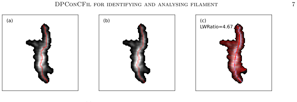
The load-bearing mechanism is the consistency-based identification rule in Section 3.1: a filament is grown from a pair of neighboring clumps whose principal-axis directions are within a 30-degree angle tolerance of the line joining them, and then extended by clumps whose perpendicular distance to that local axis is within 4 pixels (2 arcminutes). Directional consistency is the primary signal, and positional consistency lets clumps join an established axis even when their own elongation is unreliable; edge-touching clumps are excluded from the direction test but included in the distance test. Around this rule, two graph algorithms do the analysis: the skeletonization method turns each pixel in the filament region into a node of a minimum spanning tree whose edge weights favour short, bright connections, then takes the heaviest shortest path between boundary leaves as the intensity skeleton; the substructuring method builds a clump-level tree with weights combining spatial distance, velocity-channel difference, and mean intensity, and recursively extracts the longest shortest paths to separate sub-filaments that share intersection clumps.
What would settle it
Take the clump catalog from the example field, add random orientation noise to each clump's principal axis using the scatter observed between PP and PPV fits in Appendix B, and rerun DPConCFil; if the recovered filaments fragment or merge substantially, the consistency signal is not robust enough to support the claimed advantage. Alternatively, measure the fraction of true filaments recovered from synthetic PPV cubes with known axes as signal-to-noise decreases.
Extended reading notes
Core claim
The central claim is that filamentary molecular structures can be identified in the full three-dimensional PPV datacube by exploiting a local consistency between clumps and filaments: dense clumps tend to be elongated along the filament axis, and their positions tend to lie on that axis. DPConCFil encodes this as a concrete rule — for two neighboring clumps, the angle between each clump's principal axis and the line connecting the clumps must be below 30 degrees, and additional clumps must fall within 4 pixels of that line — and then merges overlapping clump records into filaments, inheriting their regions. The same package then derives intensity skeletons from a graph-theoretic minimum spanning tree weighted by distance and integrated intensity, and decomposes complex filaments into sub-filaments through a recursive longest-shortest-path procedure. The paper reports that this recovers all visually identifiable filaments in the example field, separates filaments that overlap spatially but differ by about 11 km/s in velocity, and identifies 344 filaments, containing roughly half of all clumps, in the MWISP application region.
Load-bearing premise
The method depends on a single Gaussian fit to each clump's integrated-intensity map giving a reliable orientation for the local filament axis; if those directions are noisy or biased for a substantial fraction of clumps, real filaments will be fragmented or missed.
Editorial extensions
If this is right
- Filaments that overlap on the sky but are separated in velocity, such as Filaments 1 and 7 in the example field, are kept distinct instead of being merged by velocity integration.
- Filament regions are inherited from clump masks, so derived radial profiles and FWHM values do not depend on drawing arbitrary width boundaries around skeletons.
- From MWISP 13CO data, DPConCFil yields 344 filaments (135 with five or more clumps); 80% lie within 5 km/s of a spiral-arm velocity, and filament angular length shows no significant correlation with spiral-arm separation.
- Sub-filaments extracted by the recursive decomposition share intersection clumps; in the worked example, restricting profiles to each substructure raises the profile symmetry metric SIOU from 0.68 to 0.76.
- The same pipeline applied to a synthetic PPV cube from a galactic ISM simulation recovers long filaments and places a higher fraction of clumps inside filaments (66.2%) than in the real data, suggesting the method transfers beyond MWISP.
Reading between the lines
- Beyond the paper: a quantitative benchmark against simulated cubes with known axes would settle whether the 'better suited' claim holds, since the paper's comparison with FilFinder, DisPerSE, and MST is mainly visual and descriptive.
- Beyond the paper: the default tolerances of 30 degrees and 4 pixels are tied to MWISP's angular resolution and velocity sampling, so higher-resolution or extragalactic data would likely require rescaling, and no calibration recipe is given.
- Beyond the paper: the consistency premise implies a testable prediction that clumps whose elongation is genuinely perpendicular to the local filament axis should be rare; searching for such perpendicular-clump filaments in the catalog would bound how often the key assumption fails.
- Beyond the paper: the sub-filament decomposition could serve as a quantitative definition of hubs in hub-filament systems, linking the method to core-formation studies; the paper notes intersection clumps are shared but does not exploit that connection.
Signed reviews
Editorial analysis
A structured set of objections, weighed in public.
Referee Report
Summary. The paper introduces DPConCFil, a suite of three algorithms for filament work in PPV space: a consistency-based identification method that grows filaments from neighboring clumps whose principal-axis directions align with the connecting line (TolAngle) and that then adds clumps within TolDistance of the local axis, a graph-based skeletonization method using intensity-weighted minimum spanning trees, and a graph-based sub-structuring method that recursively extracts sub-filaments. The authors apply the pipeline to MWISP 13CO data toward 10 deg <= l <= 20 deg, -5.25 deg <= b <= 5.25 deg, and -200 to 200 km/s, producing a catalog of 344 filaments and statistics on Galactic distribution, velocity gradients, profile symmetry, FWHM, and orientation. They compare the results visually with FilFinder, DisPerSE, and MST, and also apply the method to one Cloud Factory/POLARIS synthetic cube in Appendix E.
Significance. DPConCFil addresses a genuine problem: filament identification in PPV space, where velocity integration can blur or merge distinct structures and where pure 3D geometric methods have difficulty treating the velocity axis. The algorithmic description is clear, Equations (1)-(4) define the graph weights explicitly, Table 1 gives the default parameters, and the code is publicly available on GitHub and Zenodo with a manual. The substructuring method appears to improve profile symmetry relative to treating a whole complex filament as a single object, and the MWISP catalog is a useful observational product. The method is not circular: it does not derive physical parameters from assumptions that already contain the answer. However, the central claim that DPConCFil is 'better suited for identifying and analyzing filaments of various scales in the PPV space' is not yet quantitatively supported; the simulation test in Appendix E, where ground truth is available, is used only for visual comparison. A quantitative recovery analysis and a sensitivity study of the tolerances are needed before the comparative claim can be accepted.
major comments (3)
- [Section 5; Appendix E] The paper's central comparative claim, that DPConCFil is 'better suited for identifying and analyzing filaments of various scales in the PPV space' (Section 5), is supported only by side-by-side visual inspection in Figures 9, 17-19, 21, and 23. In the one case with known ground truth, the Cloud Factory/POLARIS synthetic cube in Appendix E, no recovery metrics are reported: there is no completeness, purity, false-positive rate, skeleton-position error, or clump-membership accuracy for DPConCFil or for FilFinder, DisPerSE, and MST. Because the catalog and all statistics in Section 4 inherit the identification output, the absence of a quantitative recovery test leaves the core effectiveness claim unverified. I recommend adding a recovery analysis on the Appendix E simulation, using the known filamentary structure, and reporting the same metrics for all four methods with identical parameter settings.
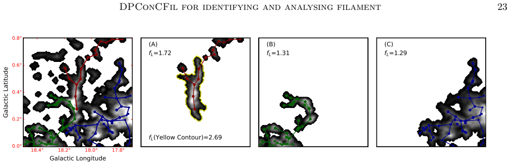
- [Section 3.1.2; Appendix B] The identification method's seed step requires two neighboring clumps whose principal-axis directions both lie within TolAngle = 30 degrees of the connecting line (Section 3.1.2). Appendix B shows that in the velocity-integrated PP map, blending of different velocity components can shift clump positions and orientations substantially; the same concern applies to PPV-space clump axes. The paper asserts that consistency is 'prevalent' in PPV space, but it does not quantify the distribution of angular offsets between clump principal axes and the true local filament axis. If a non-negligible fraction of clumps have noisy or biased axes, seed pairs will fail to form and genuine filaments will be fragmented or missed. A quantitative test on the simulated cube, such as the distribution of clump-axis offsets relative to the known local filament orientation, plus a sensitivity scan of TolAngle and TolDistance, would determine whether this failure mode is important. This is load-bearing because the entire identification criterion depends on the reliability of the clump principal-axis estimates.
- [Section 4.2; Table 3] The headline catalog statistics, including 344 filaments, 52.3% of clumps inside filaments, and the medians in Table 3, depend on three free parameters: TolAngle = 30 degrees, TolDistance = 4 pixels, and LW Ratio = 2.5. Section 3.4 states that the defaults are based on 'extensive experimental results' but gives no stability or sensitivity analysis. Since the catalog is a central deliverable, the paper should show how the filament count, clump-membership fraction, and key median properties respond to reasonable variations of these parameters. Without this, the reader cannot distinguish robust trends from threshold-dependent artifacts.
minor comments (4)
- [Section 3.2.1; Equations (1)-(2)] The graph containing all points of a filament region is named G1 in the text, but Equation (1) refers to 'the graph G2'; Section 3.3 later uses G2 for the substructure graph. Please align the notation.
- [Figure 14] The figure has duplicate and inconsistent panel labels: the second row uses (d), (e), (h) and the third row uses (d), (e), (f), while the caption says panels (a)-(f). Please re-letter all panels and update the caption and text references accordingly.
- [Throughout] There are several typographical errors: 'wight' in Equations (1)-(4), 'methonds' in the first paragraph of Section 4.1, and 'flaments' in the note to Table 2. Please proofread carefully.
- [Section 4.1; Table 2] The text notes that not all filaments in Table 2 appear in the application-data catalog because of differences in edge clumps, but the catalog table itself does not carry this caveat. A brief note in the machine-readable catalog would help users avoid misinterpreting the sample selection.
Circularity Check
Minor circularity in peripheral validation statements; central algorithm is an explicit operational definition and is not circular.
-
self definitional
[Appendix E, final paragraph]
"These experiments support the widespread consistency observed across various simulated data (Hennebelle 2013)."
The 'experiments' are DPConCFil runs on a synthetic cube. DPConCFil's identification criterion (Section 3.1.1) defines a filament as clumps whose directions and positions are consistent with the local filament axis, and Section 3.1.2 records exactly those clump pairs. Hence any filament output by DPConCFil exhibits clump-filament consistency by construction; running the algorithm cannot independently corroborate the prevalence of that consistency. The only independent support is the cited Hennebelle (2013) result. This is a peripheral overstatement rather than the paper's central method claim.
-
self definitional
[Appendix B, final paragraph]
"The clumps in Figure 2 and Figure 21 indicate that consistency between the direction and position of clumps and the local axis of the filaments in PPV space is prevalent, regardless of whether the filaments are large scale or small scale."
The filaments shown in Figure 2 (example data) and Figure 21 (GMF B and C) are those identified by DPConCFil, whose membership rule already requires directional or positional consistency with a local filament axis. Therefore the 'prevalent consistency' is guaranteed by construction of the identified sample; the figure cannot independently indicate its prevalence. The statement is used as an observational remark, not to support the central 'better suited' comparative claim, but it is circular as written.
full rationale
The paper's central contribution is an algorithm whose filament definition is explicitly operational: Section 3.1.1 defines a filament as elongated, velocity-continuous structure made of clumps whose directions or positions are consistent with a local axis, and Section 3.1.2 builds filaments by applying exactly that rule. This is a detection algorithm implementing its own stated definition, not a hidden derivation of a result from an input that contains it. The tunable parameters (TolAngle, TolDistance, LW Ratio) are thresholds, not quantities fitted to a target and then renamed as predictions; the Section 4 statistics describe the output sample and are therefore parameter-sensitive but not circular. The comparative claim that DPConCFil is 'better suited for identifying and analyzing filaments of various scales in the PPV space' (Section 5) rests on qualitative side-by-side images and lacks quantitative recovery metrics such as completeness or purity; that is a validation gap and a correctness risk, not a circular reduction. Self-citations to FacetClumps (Jiang et al. 2023) supply the input clump catalog; FacetClumps is a separately published algorithm, and using it as input is a modeling choice rather than a circular derivation. The only genuine circular steps are the two peripheral statements above, where DPConCFil's own output is used to claim support for the very consistency premise that defines its filaments. These do not undermine the central algorithmic content, so the overall circularity score is low.
Assumptions & free parameters
free parameters (3)
- TolAngle =
30 degrees
- TolDistance =
4 pixels (2 arcmin)
- LW_Ratio =
2.5
assumptions (3)
- domain assumption Clump principal-axis directions are reliable tracers of local filament orientation in PPV space.
- domain assumption Neighboring-clump connectivity, as defined by FacetClumps masks, defines the candidate graph for filament assembly.
- standard math Minimum spanning tree methods yield the optimal skeleton and sub-structure paths for a filament region.
Cite this review
Pith. "Pith review of Investigations of MWISP Filaments. I. Filament Identification and Analysis Algorithms, and Source Catalogue." pith.science (2026). https://pith.science/paper/F3NJT4D7
@misc{pith2026241201238,
  author       = {Pith},
  title        = {Pith review of: Investigations of MWISP Filaments. I. Filament Identification and Analysis Algorithms, and Source Catalogue},
  year         = {2026},
  howpublished = {\url{https://pith.science/paper/F3NJT4D7}},
  note         = {Machine review of arXiv:2412.01238}
}
abstract
Filaments play a crucial role in providing the necessary environmental conditions for star formation, actively participating in the process. To facilitate the identification and analysis of filaments, we introduce DPConCFil (Directional and Positional Consistency between Clumps and Filaments), a suite of algorithms comprising one identification method and two analysis methods. The first method, the consistency-based identification approach, uses directional and positional consistency among neighboring clumps and local filament axes to identify filaments in the PPV datacube. The second method employs a graph-based skeletonization technique to extract the filament intensity skeletons. The third method, a graph-based substructuring approach, allows the decomposition of complex filaments into simpler sub-filaments. We demonstrate the effectiveness of DPConCFil by applying the identification method to the clumps detected in the Milky Way Imaging Scroll Painting (MWISP) survey dataset by FacetClumps, successfully identifying a batch of filaments across various scales within $10^{\circ} \leq l \leq 20^{\circ}$, $-5.25^{\circ} \leq b \leq 5.25^{\circ}$ and -200 km s$^{-1}$ $\leq v \leq$ 200 km s$^{-1}$. Subsequently, we apply the analysis methods to the identified filaments, presenting a catalog with basic parameters and conducting statistics of their galactic distribution and properties. DPConCFil is openly available on GitHub, accompanied by a manual.
Figures


Figures from the paper (20 more)





Reference graph
Works this paper leans on
-
[1]
, " * write output.state after.block = add.period write newline
ENTRY address archivePrefix author booktitle chapter doi edition editor eprint howpublished institution journal key month number organization pages publisher school series title misctitle type volume year version url label extra.label sort.label short.list INTEGERS output.state before.all mid.sentence after.sentence after.block FUNCTION init.state.consts ...
-
[2]
write newline
" write newline "" before.all 'output.state := FUNCTION format.url url empty "" new.block "" url * "" * if FUNCTION format.eprint eprint empty "" archivePrefix empty "" archivePrefix "arXiv" = new.block " " eprint * " " * new.block " " eprint * " " * if if if FUNCTION format.doi doi empty "" " " doi * " " * if FUNCTION format.pid doi empty eprint empty ur...
-
[3]
- [1] #1 = = ^ ^ ^ .\!\!^ d .\!\!^ h .\!\!^ m .\!\!^ s .\!\!^ @mss
thebibliography [1] 20pt to REFERENCES 6pt =0pt -12pt 10pt plus 3pt =0pt =0pt =1pt plus 1pt =0pt =0pt -12pt =13pt plus 1pt =20pt =13pt plus 1pt \@M =10000 =-1.0em =0pt =0pt 0pt =0pt =1.0em @enumiv\@empty 10000 10000 `\.\@m \@noitemerr \@latex@warning Empty `thebibliography' environment \@ifnextchar \@reference \@latexerr Missing key on reference command E...
2021
-
[4]
2016, , 590, A131, 10.1051/0004-6361/201527674
Abreu-Vicente , J., Ragan , S., Kainulainen , J., et al. 2016, , 590, A131, 10.1051/0004-6361/201527674
-
[5]
2014, in Protostars and Planets VI, ed
Andr \'e , P., Di Francesco , J., Ward-Thompson , D., et al. 2014, in Protostars and Planets VI, ed. H. Beuther , R. S. Klessen , C. P. Dullemond , & T. Henning , 27--51, 10.2458/azu_uapress_9780816531240-ch002
-
[6]
2010, , 518, L102, 10.1051/0004-6361/201014666
Andr \'e , P., Men'shchikov , A., Bontemps , S., et al. 2010, , 518, L102, 10.1051/0004-6361/201014666
-
[7]
2013, , 553, A119, 10.1051/0004-6361/201220822
Arzoumanian , D., Andr \'e , P., Peretto , N., & K \"o nyves , V. 2013, , 553, A119, 10.1051/0004-6361/201220822
-
[8]
2011, , 529, L6, 10.1051/0004-6361/201116596
Arzoumanian , D., Andr \'e , P., Didelon , P., et al. 2011, , 529, L6, 10.1051/0004-6361/201116596
Show all 91 references
-
[9]
2019, , 621, A42, 10.1051/0004-6361/201832725
Arzoumanian , D., Andr \'e , P., K \"o nyves , V., et al. 2019, , 621, A42, 10.1051/0004-6361/201832725
2019 doi
-
[10]
M., Sip o cz , B
Astropy Collaboration , Price-Whelan , A. M., Sip o cz , B. M., et al. 2018, , 156, 123, 10.3847/1538-3881/aabc4f
2018 doi
-
[11]
N., Offner , S
Beaumont , C. N., Offner , S. S. R., Shetty , R., Glover , S. C. O., & Goodman , A. A. 2013, , 777, 173, 10.1088/0004-637X/777/2/173
2013 doi
-
[12]
Berry , D. S. 2015, Astronomy and Computing, 10, 22, 10.1016/j.ascom.2014.11.004
2015 doi
-
[13]
2017, , 601, A90, 10.1051/0004-6361/201629001
Brauer , R., Wolf , S., Reissl , S., & Ober , F. 2017, , 601, A90, 10.1051/0004-6361/201629001
2017 doi
-
[14]
M., et al
Bresnahan , D., Ward-Thompson , D., Kirk , J. M., et al. 2018, , 615, A125, 10.1051/0004-6361/201730515
2018 doi
-
[15]
S., Montier , L., Ferri \`e re , K., & Ristorcelli , I
Carri \`e re , J. S., Montier , L., Ferri \`e re , K., & Ristorcelli , I. 2022, , 668, A41, 10.1051/0004-6361/202243506
2022 doi
-
[17]
2020 b , , 891, 84, 10.3847/1538-4357/ab7378
---. 2020 b , , 891, 84, 10.3847/1538-4357/ab7378
2020 doi
-
[18]
2023 a , , 165, 16, 10.3847/1538-3881/ac9ea2
Chen , X., Sun , L., Feng , J., et al. 2023 a , , 165, 16, 10.3847/1538-3881/ac9ea2
2023 doi
-
[19]
2023 b , , 525, 107, 10.1093/mnras/stad2259
Chen , Z., Sefako , R., Yang , Y., et al. 2023 b , , 525, 107, 10.1093/mnras/stad2259
2023 doi
-
[20]
J., Debattista , V
Clarke , A. J., Debattista , V. P., Ro s kar , R., & Quinn , T. 2017, , 465, L79, 10.1093/mnrasl/slw214
2017 doi
-
[21]
D., Whitworth , A
Clarke , S. D., Whitworth , A. P., Spowage , R. L., et al. 2018, , 479, 1722, 10.1093/mnras/sty1675
2018 doi
-
[22]
D., Williams , G
Clarke , S. D., Williams , G. M., & Walch , S. 2020, , 497, 4390, 10.1093/mnras/staa2298
2020 doi
-
[23]
Cox , N. L. J., Arzoumanian , D., Andr \'e , P., et al. 2016, , 590, A110, 10.1051/0004-6361/201527068
2016 doi
-
[24]
J., Hacar , A., Clark , S
Feng , J., Smith , R. J., Hacar , A., Clark , S. E., & Seifried , D. 2024, , 528, 6370, 10.1093/mnras/stae407
2024 doi
-
[25]
2022, , 259, 36, 10.3847/1538-4365/ac4a76
Ge , Y., & Wang , K. 2022, , 259, 36, 10.3847/1538-4365/ac4a76
2022 doi
-
[26]
2023, , 675, A119, 10.1051/0004-6361/202245784
Ge , Y., Wang , K., Duarte-Cabral , A., et al. 2023, , 675, A119, 10.1051/0004-6361/202245784
2023 doi
-
[27]
1974, , 189, 441, 10.1086/152821
Goldreich , P., & Kwan , J. 1974, , 189, 441, 10.1086/152821
1974 doi
-
[28]
2017, , 834, 202, 10.3847/1538-4357/834/2/202
Gritschneder , M., Heigl , S., & Burkert , A. 2017, , 834, 202, 10.3847/1538-4357/834/2/202
2017 doi
- [29]
-
[30]
2013, , 554, A55, 10.1051/0004-6361/201220090
Hacar , A., Tafalla , M., Kauffmann , J., & Kov \'a cs , A. 2013, , 554, A55, 10.1051/0004-6361/201220090
2013 doi
-
[31]
J., & Schult , D
Hagberg , A., Swart , P. J., & Schult , D. A. 2008, Proceedings of the 7th Python in Science Conference (SciPy2008). https://www.osti.gov/biblio/960616
2008
-
[32]
2007, , 654, 988, 10.1086/509321
Hartmann , L., & Burkert , A. 2007, , 654, 988, 10.1086/509321
2007 doi
-
[33]
2013, , 556, A153, 10.1051/0004-6361/201321292
Hennebelle , P. 2013, , 556, A153, 10.1051/0004-6361/201321292
2013 doi
-
[34]
2019, Frontiers in Astronomy and Space Sciences, 6, 5, 10.3389/fspas.2019.00005
Hennebelle , P., & Inutsuka , S.-i. 2019, Frontiers in Astronomy and Space Sciences, 6, 5, 10.3389/fspas.2019.00005
2019
-
[35]
Hunter , J. D. 2007, Computing in Science and Engineering, 9, 90, 10.1109/MCSE.2007.55
2007 doi
-
[36]
2016, , 833, 10, 10.3847/0004-637X/833/1/10
Inoue , T., & Inutsuka , S.-i. 2016, , 833, 10, 10.3847/0004-637X/833/1/10
2016 doi
-
[37]
F., Smith , R
Izquierdo , A. F., Smith , R. J., Glover , S. C. O., et al. 2021, , 500, 5268, 10.1093/mnras/staa3470
2021 doi
-
[38]
M., Finn , S
Jackson , J. M., Finn , S. C., Chambers , E. T., Rathborne , J. M., & Simon , R. 2010, , 719, L185, 10.1088/2041-8205/719/2/L185
2010 doi
-
[39]
2024, DPConCFil: A Collection of Filament Identification and Analysis Algorithms , Zenodo, 10.5281/zenodo.13853675
Jiang, Y. 2024, DPConCFil: A Collection of Filament Identification and Analysis Algorithms , Zenodo, 10.5281/zenodo.13853675
2024 doi
-
[40]
2023, , 267, 32, 10.3847/1538-4365/acda89
Jiang , Y., Chen , Z., Zheng , S., et al. 2023, , 267, 32, 10.3847/1538-4365/acda89
2023 doi
-
[41]
2022, Astronomy and Computing, 100613, https://doi.org/10.1016/j.ascom.2022.100613
Jiang, Y., Zheng, S., Jiang, Z., et al. 2022, Astronomy and Computing, 100613, https://doi.org/10.1016/j.ascom.2022.100613
2022
-
[42]
W., & Rosolowsky , E
Koch , E. W., & Rosolowsky , E. W. 2015, , 452, 3435, 10.1093/mnras/stv1521
2015 doi
-
[43]
Koda , J., Sawada , T., Hasegawa , T., & Scoville , N. Z. 2006, , 638, 191, 10.1086/498640
2006 doi
-
[44]
2015, , 584, A91, 10.1051/0004-6361/201525861
K \"o nyves , V., Andr \'e , P., Men'shchikov , A., et al. 2015, , 584, A91, 10.1051/0004-6361/201525861
2015 doi
-
[46]
2020 b , , 635, A34, 10.1051/0004-6361/201834753
---. 2020 b , , 635, A34, 10.1051/0004-6361/201834753
2020 doi
-
[47]
2020, , 638, A74, 10.1051/0004-6361/201936442
Ladjelate , B., Andr \'e , P., K \"o nyves , V., et al. 2020, , 638, A74, 10.1051/0004-6361/201936442
2020 doi
-
[48]
S., Leurini , S., et al
Li , G.-X., Urquhart , J. S., Leurini , S., et al. 2016, , 591, A5, 10.1051/0004-6361/201527468
2016 doi
- [49]
-
[50]
S., Lopez-Rodriguez , E., Soam , A., & Klein , R
Li , P. S., Lopez-Rodriguez , E., Soam , A., & Klein , R. I. 2022, , 514, 3024, 10.1093/mnras/stac1527
2022 doi
-
[51]
2018, , 619, A166, 10.1051/0004-6361/201833406
Mattern , M., Kauffmann , J., Csengeri , T., et al. 2018, , 619, A166, 10.1051/0004-6361/201833406
2018 doi
-
[52]
2013, , 560, A63, 10.1051/0004-6361/201321885
Men'shchikov , A. 2013, , 560, A63, 10.1051/0004-6361/201321885
2013 doi
-
[53]
2010, , 518, L103, 10.1051/0004-6361/201014668
Men'shchikov , A., Andr \'e , P., Didelon , P., et al. 2010, , 518, L103, 10.1051/0004-6361/201014668
2010 doi
-
[54]
2018, , 56, 41, 10.1146/annurev-astro-091916-055235
Motte , F., Bontemps , S., & Louvet , F. 2018, , 56, 41, 10.1146/annurev-astro-091916-055235
2018 doi
-
[55]
Myers , P. C. 2009, , 700, 1609, 10.1088/0004-637X/700/2/1609
2009 doi
-
[56]
Oliphant , T. E. 2007, Computing in Science and Engineering, 9, 10, 10.1109/MCSE.2007.58
2007 doi
-
[57]
2016, , 455, 1134, 10.1093/mnras/stv2380
Pakmor , R., Springel , V., Bauer , A., et al. 2016, , 455, 1134, 10.1093/mnras/stv2380
2016 doi
-
[58]
V., Psaradaki , I., Skalidis , R., Tassis , K., & Andrews , J
Panopoulou , G. V., Psaradaki , I., Skalidis , R., Tassis , K., & Andrews , J. J. 2017, , 466, 2529, 10.1093/mnras/stw3060
2017 doi
-
[59]
V., Tassis , K., Goldsmith , P
Panopoulou , G. V., Tassis , K., Goldsmith , P. F., & Heyer , M. H. 2014, , 444, 2507, 10.1093/mnras/stu1601
2014 doi
-
[60]
2011, Journal of Machine Learning Research, 12, 2825
Pedregosa, F., Varoquaux, G., Gramfort, A., et al. 2011, Journal of Machine Learning Research, 12, 2825
2011
-
[61]
2012, , 541, A63, 10.1051/0004-6361/201118663
Peretto , N., Andr \'e , P., K \"o nyves , V., et al. 2012, , 541, A63, 10.1051/0004-6361/201118663
2012 doi
-
[62]
E., Arzoumanian , D., Andre , P., et al
Pineda , J. E., Arzoumanian , D., Andre , P., et al. 2023, in Astronomical Society of the Pacific Conference Series, Vol. 534, Protostars and Planets VII, ed. S. Inutsuka , Y. Aikawa , T. Muto , K. Tomida , & M. Tamura , 233, 10.48550/arXiv.2205.03935
-
[63]
E., Henning , T., Tackenberg , J., et al
Ragan , S. E., Henning , T., Tackenberg , J., et al. 2014, , 568, A73, 10.1051/0004-6361/201423401
2014 doi
-
[64]
J., Menten , K
Reid , M. J., Menten , K. M., Brunthaler , A., et al. 2019, , 885, 131, 10.3847/1538-4357/ab4a11
2019 doi
-
[65]
2016, , 593, A87, 10.1051/0004-6361/201424930
Reissl , S., Wolf , S., & Brauer , R. 2016, , 593, A87, 10.1051/0004-6361/201424930
2016 doi
-
[66]
K., Ginsburg , A., et al
Rosolowsky , E., Dunham , M. K., Ginsburg , A., et al. 2010, , 188, 123, 10.1088/0067-0049/188/1/123
2010 doi
-
[67]
W., Pineda , J
Rosolowsky , E. W., Pineda , J. E., Kauffmann , J., & Goodman , A. A. 2008, , 679, 1338, 10.1086/587685
2008 doi
-
[68]
J., Richer , J
Salji , C. J., Richer , J. S., Buckle , J. V., et al. 2015, , 449, 1782, 10.1093/mnras/stv369
2015 doi
-
[69]
Schisano , E., Rygl , K. L. J., Molinari , S., et al. 2014, , 791, 27, 10.1088/0004-637X/791/1/27
2014 doi
-
[70]
L., van der Tak , F
Sch \"o ier , F. L., van der Tak , F. F. S., van Dishoeck , E. F., & Black , J. H. 2005, , 432, 369, 10.1051/0004-6361:20041729
2005 doi
- [71]
-
[72]
2019, , 632, A83, 10.1051/0004-6361/201935689
Shimajiri , Y., Andr \'e , P., Ntormousi , E., et al. 2019, , 632, A83, 10.1051/0004-6361/201935689
2019 doi
-
[73]
J., Glover , S
Smith , R. J., Glover , S. C. O., & Klessen , R. S. 2014, , 445, 2900, 10.1093/mnras/stu1915
2014 doi
-
[74]
J., Glover , S
Smith , R. J., Glover , S. C. O., Klessen , R. S., & Fuller , G. A. 2016, , 455, 3640, 10.1093/mnras/stv2559
2016 doi
-
[75]
J., Tre , R
Smith , R. J., Tre , R. G., Sormani , M. C., et al. 2020, , 492, 1594, 10.1093/mnras/stz3328
2020 doi
-
[77]
2011, , 414, 384, 10.1111/j.1365-2966.2011.18395.x
Sousbie , T., Pichon , C., & Kawahara , H. 2011, , 414, 384, 10.1111/j.1365-2966.2011.18395.x
2011
-
[78]
2010, , 401, 791, 10.1111/j.1365-2966.2009.15715.x
Springel , V. 2010, , 401, 791, 10.1111/j.1365-2966.2009.15715.x
2010
-
[79]
2019, , 240, 9, 10.3847/1538-4365/aaf1c8
Su , Y., Yang , J., Zhang , S., et al. 2019, , 240, 9, 10.3847/1538-4365/aaf1c8
2019 doi
-
[80]
2019, , 623, A142, 10.1051/0004-6361/201834049
Suri , S., S \'a nchez-Monge , \'A ., Schilke , P., et al. 2019, , 623, A142, 10.1051/0004-6361/201834049
2019 doi
-
[81]
2015, , 574, A104, 10.1051/0004-6361/201424576
Tafalla , M., & Hacar , A. 2015, , 574, A104, 10.1051/0004-6361/201424576
2015 doi
-
[82]
P., Fuente , A., S \'a nchez-Monge , \'A ., et al
Trevi \ n o-Morales , S. P., Fuente , A., S \'a nchez-Monge , \'A ., et al. 2019, , 629, A81, 10.1051/0004-6361/201935260
2019 doi
-
[83]
L., Nunez-Iglesias , J., et al
van der Walt, S., S ch\"onberger, J. L., Nunez-Iglesias , J., et al. 2014, PeerJ, 2, e453, 10.7717/peerj.453
2014 doi
-
[84]
C., & Zamora-Avil \'e s , M
V \'a zquez-Semadeni , E., Palau , A., Ballesteros-Paredes , J., G \'o mez , G. C., & Zamora-Avil \'e s , M. 2019, , 490, 3061, 10.1093/mnras/stz2736
2019 doi
-
[85]
2024, , 686, L11, 10.1051/0004-6361/202450296
Wang , K., Ge , Y., & Baug , T. 2024, , 686, L11, 10.1051/0004-6361/202450296
2024 doi
-
[86]
2016, , 226, 9, 10.3847/0067-0049/226/1/9
Wang , K., Testi , L., Burkert , A., et al. 2016, , 226, 9, 10.3847/0067-0049/226/1/9
2016 doi
-
[87]
J., Falle , S
Wareing , C. J., Falle , S. A. E. G., & Pittard , J. M. 2019, , 485, 4686, 10.1093/mnras/stz768
2019 doi
-
[88]
2021, , 257, 51, 10.3847/1538-4365/ac242a
Yuan , L., Yang , J., Du , F., et al. 2021, , 257, 51, 10.3847/1538-4365/ac242a
2021 doi
-
[89]
2016, Research in Astronomy and Astrophysics, 16, 56, 10.1088/1674-4527/16/4/056
Zhan , X.-L., Jiang , Z.-B., Chen , Z.-W., Zhang , M.-M., & Song , C. 2016, Research in Astronomy and Astrophysics, 16, 56, 10.1088/1674-4527/16/4/056
2016 doi
-
[90]
2024, , 689, A3, 10.1051/0004-6361/202449853
Zhang , G.-Y., Andr \'e , P., Men'shchikov , A., & Li , J.-Z. 2024, , 689, A3, 10.1051/0004-6361/202449853
2024 doi
-
[91]
2020, , 642, A76, 10.1051/0004-6361/202037721
Zhang , G.-Y., Andr \'e , P., Men'shchikov , A., & Wang , K. 2020, , 642, A76, 10.1051/0004-6361/202037721
2020 doi
-
[92]
2018, , 864, 153, 10.3847/1538-4357/aacc66
Zucker , C., Battersby , C., & Goodman , A. 2018, , 864, 153, 10.3847/1538-4357/aacc66
2018 doi
-
[93]
Zucker , C., & Chen , H. H.-H. 2018, , 864, 152, 10.3847/1538-4357/aad3b5
2018 doi
-
[94]
2019, , 887, 186, 10.3847/1538-4357/ab517d
Zucker , C., Smith , R., & Goodman , A. 2019, , 887, 186, 10.3847/1538-4357/ab517d
2019 doi
Reviewed August 12, 2026 · model on record in the stance chip above.
Discussion (0). Continue with ORCID to comment.