REVIEW 4 major objections 7 minor 18 references
Signal denoising based on the Schr\"odinger operator's eigenspectrum and a curvature constraint
T0 review · 4 major / 7 minor · reviewed 2026-08-14 · deepseek-v4-flash
Pith's one-line read A curvature penalty lets Schrödinger-operator denoising preserve pulse peaks without requiring peak locations or noise-region priors.
desk verdict C-SCSA is a plausible incremental extension of the authors' SCSA denoiser, but the curvature-penalty justification does not actually transfer from the noisy input to the reconstruction, so the peak-preservation claim should be read as an empirical observation, not a proven guarantee. read the letter →
The pith
A machine-rendered reading of the paper's core claim, the machinery that carries it, and where it could break.
The reading
What carries the argument
The central object is the Schrödinger operator $-h^2 \frac{d^2\psi}{dt^2} - y(t)\psi = \lambda\psi$, with the noisy signal acting as the potential. Its negative eigenvalues $\lambda_{nh} = -\kappa_{nh}^2$ and the associated $L^2$-normalized eigenfunctions $\psi_{nh}$ are used to reconstruct the signal as $y_h(t) = 4h \sum_{n=1}^{N_h} \kappa_{nh} \psi_{nh}^2(t)$. The semiclassical parameter $h$ controls how many eigenfunctions are retained, and the curvature constraint $k(t) = |y_h''(t)|/(1 + y_h'(t)^2)^{3/2}$ is the mechanism that selects $h$. The load-bearing identity is Proposition 1's formula, which gives the expected curvature of adjacent differences as an integral that grows with the noise variance, thereby connecting larger noise to larger curvature and motivating the penalty term in the cost function.
What would settle it
Generate a signal with sharp true spikes whose curvature is comparable to or larger than the curvature of the added noise, run C-SCSA at noise levels from 1% to 12%, and measure peak height and width relative errors. If the errors are as large as those of Savitzky-Golay filtering, the claim that C-SCSA guarantees peak preservation fails. Alternatively, compare the curvature of the chosen $y_h$ to the curvature of the true signal: if the reconstructed curvature is systematically lower for signals with genuinely high-curvature features, the curvature penalty is over-smoothing beyond noise removal.
Extended reading notes
Core claim
The central claim is that selecting the semiclassical parameter $h$ by minimizing a cost function that combines fidelity to the noisy signal with a curvature penalty on the reconstruction yields a denoiser that removes noise without flattening peaks. Specifically, the paper defines $J = \|y_\delta - y_h\|_2^2 + \mu \int |k(t)|\,dt$, where $k(t)$ is the curvature of the reconstructed signal, and then scans $h$ to minimize this cost. The supporting theoretical result, Proposition 1, derives an expression for the expected curvature of adjacent differences in the noisy signal and shows that this expectation increases with the noise variance; the paper uses this to justify penalizing curvature as a noise-reduction mechanism. Numerically, C-SCSA reports lower peak-height and peak-width relative errors than the comparison methods on single Gaussian peaks, and higher or comparable post-denoising SNR on simulated multi-peak signals, real-noise ECG records, and several standard test signals, especially when the signal is regular and slowly varying.
Load-bearing premise
The proof shows that adjacent differences in the noisy input have larger expected curvature when noise increases, but the algorithm actually penalizes the curvature of the reconstructed signal; the paper does not prove that these two curvatures are equivalent or that minimizing the latter removes the former.
Editorial extensions
If this is right
- C-SCSA can be applied to pulse-shaped signals without needing to locate peaks or identify noise-dominant intervals, unlike the earlier α-SCSA method.
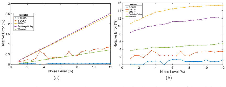
- On single Gaussian peaks with 1–12% Gaussian noise, C-SCSA reports lower peak-height and peak-width relative errors than EMD-IT, Savitzky-Golay, and wavelet denoising.
- On multi-peak simulated signals and real-noise ECG records from the MIT-BIH database, C-SCSA achieves SNR after denoising that is competitive with or better than Savitzky-Golay and EMD-IT, and comparable to the wavelet method.
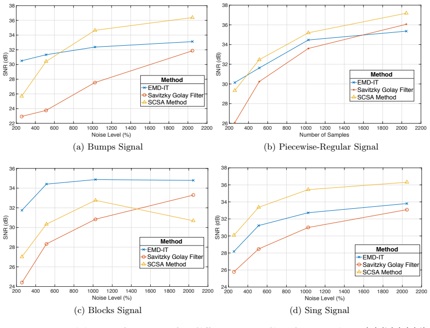
- On piecewise-regular, Doppler, blocks, bumps, and sing test signals, C-SCSA outperforms EMD-IT and Savitzky-Golay for regular and slowly varying cases, and remains effective across sampling frequencies from 256 to 2048 samples.
- Because the cost function operates on the whole signal, C-SCSA extends SCSA-based denoising beyond magnetic resonance spectroscopy to a broader class of biomedical and spectral signals.
Reading between the lines
- The curvature-based rule suggests a general principle for spectral denoising: choose the decomposition threshold by minimizing fidelity plus a geometric regularity term, which could also be applied to wavelet coefficient selection or EMD interval thresholding.
- Proposition 1's relation between adjacent-difference curvature and noise variance could be inverted to estimate the noise level from a single noisy record, allowing the smoothing parameter $\mu$ to be set automatically rather than by an order-of-magnitude scan.
- The method's dependence on reconstruction curvature implies it may over-smooth signals whose true features have curvature comparable to noise, such as very sharp spikes or edges; testing on such signals would reveal the boundary of the peak-preservation claim.
- Viewing the curvature penalty as a form of total-variation or mean-curvature flow could connect C-SCSA to nonlinear diffusion denoising and potentially yield convergence guarantees that the paper does not provide.
Signed reviews
Editorial analysis
A structured set of objections, weighed in public.
Referee Report
Summary. The manuscript proposes C-SCSA, a denoising method that augments semi-classical signal analysis (SCSA) with a curvature penalty. Section 3 defines the cost function Jbar = sum_i [y_delta(t_i) - y_h(t_i)]^2 + mu sum_i k(t_i), where k(t_i) is the curvature of the SCSA reconstruction y_h, and Proposition 1 computes the expected curvature of adjacent differences of the noisy input under a zero-mean jointly Gaussian model, showing that this expectation increases with the noise variance. The algorithm then scans the semi-classical parameter h to minimize Jbar. Section 4 evaluates C-SCSA against Savitzky-Golay, wavelet, and EMD-IT denoising on single- and multi-peak Gaussian signals, ECG records corrupted with real noise from the MIT-BIH database, and standard test signals (Doppler, piecewise-regular, blocks, bumps) at multiple noise levels and sampling frequencies. The paper claims that C-SCSA preserves peak height and width and outperforms or matches the baselines.
Significance. The paper addresses a practically relevant problem: denoising pulse-shaped signals without peak-localization priors. The C-SCSA cost function is a reasonable extension of SCSA, and the simulation protocol is detailed, including multiple signals, noise levels, sampling frequencies, and a real-noise ECG test against three baselines. Proposition 1 is a nontrivial calculation, and the appendix derivation is internally consistent. However, the central theoretical link from noise-driven curvature of the input to a penalty on the reconstruction's curvature is not established, and the parameter selection uses oracle knowledge of the clean signal. As presented, the claimed guarantee of peak preservation is not supported, so the significance is conditional on additional analysis and validation.
major comments (4)
- [Section 3, Eqs. (5)-(10) and Proposition 1] The theoretical support for the curvature penalty is derived for the adjacent differences x_m and w_m of the noisy input y_delta under a zero-mean jointly Gaussian model (Eq. 7), but the penalty in Eq. (10) is applied to the curvature k(t_i) of the SCSA reconstruction y_h. The paper does not provide a lemma or estimate showing that penalizing the reconstruction's curvature is equivalent to, or even correlated with, reducing the input curvature caused by noise. Because signal peaks have high curvature, the penalty can suppress the very features the method claims to preserve; therefore the statement in Section 5 that C-SCSA 'guarantees the peaks are well preserved' is not justified by Proposition 1. Either supply a transfer argument relating curvature of y_h to noise in y_delta, or reword the claim and support peak preservation empirically over a range of mu and h.
- [Section 4.2, parameter selection paragraph] The description 'we optimize each method's parameter at noise level 5%, where we iteratively optimize its parameter using the noisy signal and true signal' means that mu (and h) for C-SCSA, as well as baseline parameters, are chosen with the true clean signal. This is oracle tuning: it does not correspond to a deployable procedure when the clean signal is unknown, and it weakens the claim that C-SCSA does not need to locate signal peaks or know the noise level. The paper should either specify a fully data-driven selection rule for mu (the current rule involving max{|y_delta|} * sum k(i) * 10^nu leaves nu unspecified) or present the comparison as an oracle-parameter study and discuss behavior when parameters are selected without the clean signal.
- [Section 4.3, ECG experiments] SCSA is defined for a real positive potential y(t) (Section 2.1 and Eq. 2), yet the ECG records shown in Fig. 5 have amplitudes ranging from about -200 to 400, i.e., they contain negative values. The paper never states how the potential is made positive before computing the Schrodinger spectrum. If a baseline shift is applied, it should be described and its effect on the reported SNR improvements quantified; without this, the eigenvalue problem and the reconstruction in Eq. (1) are not well defined for these signals.
- [Section 4.2, Fig. 3] The peak-preservation experiment is performed on a single simulated Gaussian peak, and no repeated noise realizations or error bars are reported for the peak-height and peak-width relative errors; the text elsewhere reports ensemble averages over 90 realizations. Consequently, the claimed superiority of C-SCSA in peak preservation could reflect a single noise draw rather than a stable advantage. Repeating the experiment over multiple noise realizations and reporting mean plus or minus standard deviation (or box plots) is necessary to support the central peak-preserving claim.
minor comments (7)
- [Eq. (10)] The summation lower limit is written as 'i = i' and should be 'i = 1'.
- [Eq. (4)] The sign of the alpha * |SNR_yh| term in the alpha-SCSA cost appears inconsistent with minimization: if a larger SNR is desirable, adding a positive SNR term increases the cost for better reconstructions. Clarify whether the term should be negative or should be alpha / SNR_yh.
- [Fig. 4 caption] The caption states that the noise level ranges between 0.1% and 15% with interval 0.1%, but the horizontal axis shows values from 1 to 10, and the preceding paragraph describes a 1% to 12% range. Please make the range and units consistent.
- [Figs. 6 and 7 captions] The x-axis labels are inconsistent with the experiments: Fig. 6 labels the x-axis 'Noise Level (%)' while the text indicates noise levels 7%-15%, and Fig. 7 panels show both 'Noise Level (%)' and 'Number of Samples' on the x-axis although the text describes a sampling-frequency experiment. Correct all axis labels, legends, and figure cross-references.
- [Fig. 8 caption] Both panels (b) and (c) in the caption are described as 'C-SCSA denoising', but the surrounding text states that alpha-SCSA failed on the piecewise-regular signal. Clarify which panel shows alpha-SCSA and which shows C-SCSA.
- [Section 4.4, cross-references] The text cites 'Fig. 7(a) and (d)' and 'Fig. 8(a)(b)(c)(d)' in a way that does not match the figures' content; all figure cross-references should be checked and updated.
- [Section 4.2, Savitzky-Golay settings] The Savitzky-Golay parameters differ between Fig. 3 (window 29, degree 4) and Fig. 4 (filter length 17, order 4); the manuscript should explain why different settings are used in the two experiments or use a single configuration.
Circularity Check
No circular derivation: C-SCSA is validated on external benchmarks; the curvature-penalty justification is a missing transfer step, not a circular reduction.
full rationale
The paper's claimed contribution is the C-SCSA cost function, Eq. (10): J-bar = sum_i [y_delta(t_i) - y_h(t_i)]^2 + mu sum_i k(t_i), where y_h is the SCSA reconstruction from Eqs. (1)-(2). The SCSA reconstruction itself is imported from the authors' prior work, but that prior work is an independent published spectral-theoretic result with stated assumptions, not a parameter fitted to the present target data. The denoising claims are tested against external benchmarks: synthetic Gaussian peaks with known clean signals, MIT-BIH ECG records with real noise, and standard test signals (Doppler, Blocks, Bumps, Piecewise-Regular, Sing). No fitted parameter or subset of the target data is renamed as a prediction; the reported SNRs and MSEs are measured against known ground truth. The one theoretical result, Proposition 1 (Eq. 9), derives that the expected curvature of adjacent differences of the noisy input y_delta increases with noise variance. The algorithm, however, penalizes the curvature of the reconstructed signal y_h. No lemma transfers the Proposition's monotonicity from the input's adjacent differences to the curvature of y_h, so the link between the theorem and the cost function is assumed rather than derived. This is a logical gap or correctness risk, not a circular reduction: the penalty is not defined in terms of the quantity being predicted, and the 'guarantee' of peak preservation in the abstract and conclusion is an empirical observation from Fig. 3 rather than a theorem derived from the paper's own inputs. The parameter selection for baselines is a tuning/evaluation issue, not a circularity in the derivation chain. Accordingly, no circular step is present; the score is 0.
Assumptions & free parameters
free parameters (2)
- Semi-classical parameter h =
No single optimum reported; scanned or iteratively decreased to minimize the cost function, with example values 100…
- Curvature penalty weight μ =
Signal-dependent; set by max{|yδ(ti)|} Σk(i) · 10^ν with ν∈Z, and refined by scanning per signal and noise level
assumptions (5)
- domain assumption The Schrödinger operator reconstruction formula y_h = 4h Σ κ_nh ψ_nh^2 converges to the signal as h tends to zero, and higher-order eigenfunctions mainly reconstruct noise.
- domain assumption The input signal y(t) is positive, as required for the SCSA reconstruction formula in Eq. (1).
- domain assumption Adjacent differences x_m = y_{m+1} - y_m and w_m = y_m - y_{m-1} are jointly Gaussian, zero-mean, with equal variance σ_m^2 and small correlation ρ_m.
- domain assumption Noise variance in homogeneous signal regions satisfies σ_m^2 ≈ 2 σ_noise^2.
- domain assumption The finite-difference approximation of curvature in Eq. (8) adequately represents the continuous curvature defined in Eq. (6).
Cite this review
Pith. "Pith review of Signal denoising based on the Schr\"odinger operator's eigenspectrum and a curvature constraint." pith.science (2026). https://pith.science/paper/FB6N6CQ4
@misc{pith2026190807758,
  author       = {Pith},
  title        = {Pith review of: Signal denoising based on the Schr\"odinger operator's eigenspectrum and a curvature constraint},
  year         = {2026},
  howpublished = {\url{https://pith.science/paper/FB6N6CQ4}},
  note         = {Machine review of arXiv:1908.07758}
}
read the original abstract
Recently, a new Signal processing method, named Semi-Classical Signal Analysis (SCSA), has been proposed for denoising Magnetic Resonance Spectroscopy (MRS) signals. It is based on the Schr\"odinger Operator's eigenspectrum. It allows an efficient noise reduction while preserving MRS signal's peaks. In this paper, we propose to extend this approach to different signals, in particular pulse shaped signals, by including an optimization that considers curvature constraints. The performance of the method is measured by analyzing noisy signal data and comparing with other denoising methods. Results indicate that the proposed method not only produces good denoising performance but also guarantees the peaks are well preserved in the denoising process.
Figures



Figures from the paper (8 more)





Reference graph
Works this paper leans on
-
[1]
Spectral data de-noising using semi- classical signal analysis: application to localized MRS
T. M. Laleg-Kirati, J. Zhang, E. Achten, and H. Serrai, "Spectral data de-noising using semi- classical signal analysis: application to localized MRS”, NMR Biomed, vol.29, pp. 1477-1485, 2016
work page 2016
-
[2]
Semi-classical signal analysis
T. M. Laleg-Kirati, E. Crépeau, M. Sorine, "Semi-classical signal analysis”, Math. Control Signals Syst, 2013
work page 2013
-
[3]
Arterial blood pressure analysis based on scattering transform II
T. M. Laleg-Kirati, Medigue. C, Cottin F, Sorine. M, "Arterial blood pressure analysis based on scattering transform II”, Proceedings of EMBC Sciences and Technologies for Health, Lyon, France, pp. 3618-3629, 2007
work page 2007
-
[4]
T. M. Laleg-Kirati, C. Medigue, Y. Papelier, et al, "Validation of a semi-classical signal analysis method for stroke volume variation assessment: A comparison with the PiCCO technique Ann Biomed Eng”, vol.38, pp. 3618-3629, 2010
work page 2010
-
[5]
Residual Water Suppression Using the Squared Eigenfunctions of the Schrodinger Operator
A. Chahid, S. Bhaduri, M. Maoui, R Achten H. Serrai and T.M. Laleg-Kirati, "Residual Water Suppression Using the Squared Eigenfunctions of the Schrodinger Operator ", IEEE access, Vol. 9, 69126–69137, 2019. 24
work page 2019
-
[6]
A. Chahid,T. N. Alotaiby, S. Alshebeili and T-M Laleg-Kirati, "Feature Generation and Di- mensionality Reduction using the Discrete Spectrum of the Schrödinger Operator for Epileptic Spikes Detection", In Proceeding IEEE EMBC July 2019
work page 2019
-
[7]
Width Based Quantitation of Chromatographic Peaks: Principles and Principal Characteristics
A. F. Kadjo, P. K. Dasgupta, J. Su, S. Y. Liu, and K. G. Kraiczek, "Width Based Quantitation of Chromatographic Peaks: Principles and Principal Characteristics”, Analytical Chemistry, vol. 89 no.7, pp. 3884-3892, 2017
work page 2017
- [8]
Show all 18 references
-
[9]
Denoising an image by denoising its curvature image
M. Bertalmío, S. Levine, "Denoising an image by denoising its curvature image”, SIAM J. Imag. Sci., vol. 7, no. 2, pp. 187-201, 2014
2014
-
[10]
High frequency noise removal from ECG using moving average filters
V. Pandey and V. K. Giri, "High frequency noise removal from ECG using moving average filters”, International Conference on Emerging Trends in Electrical Electronics & Sustainable Energy Systems (ICETEESES), Sultanpur, pp. 191-195, 2016
2016
-
[11]
Review and comparison of smoothing algorithms for one- dimensional data noise reduction
P. Kowalski and R. Smyk, "Review and comparison of smoothing algorithms for one- dimensional data noise reduction”, 2018 International Interdisciplinary PhD Workshop (IIPhDW), Swinoujście, pp. 277-281, 2018
2018
-
[12]
Smoothing and Differentiation of Data by Simplified Least Squares Procedures
Abraham. Savitzky and M. J. E. Golay, "Smoothing and Differentiation of Data by Simplified Least Squares Procedures”, Analytical Chemistry, vol. 36, no. 8, pp. 1627-1639, 1964
1964
-
[13]
Application of adaptive Savitzky–Golay filter for EEG signal processing
D. Acharya, A. Rani, S. Agarwal, V. Singh, "Application of adaptive Savitzky–Golay filter for EEG signal processing”, Perspectives in Science, vol. 8, pp. 677-679, 2016
2016
-
[14]
Nonlineardiffusionfilteringforpeak-preservingsmoothingofaspectrum signal
Y.Li, Y.Ding, T.Li, "Nonlineardiffusionfilteringforpeak-preservingsmoothingofaspectrum signal”, Chemometrics and Intelligent Laboratory Systems, vol. 156, pp. 157-165, 2016
2016
-
[15]
Optimizing Savitzky-Golay parameters for improving spectral resolution and quantification in infrared spectroscopy
B. Zimmermann, A. Kohler, "Optimizing Savitzky-Golay parameters for improving spectral resolution and quantification in infrared spectroscopy”, Appl. Spectrosc, vol. 67, pp. 892-902, 2013. 25
2013
-
[16]
Optimal selection of wavelet basis function applied to ECG signal denoising
B. N. Singh, A. K. Tiwari, "Optimal selection of wavelet basis function applied to ECG signal denoising”, Digital Signal Processing, vol. 16, no. 3, pp. 275-287, 2006
2006
-
[17]
PhysioBank, PhysioToolkit, and PhysioNet: components of a new research resource for complex physiologic signals
A. L. Goldberger, L. A. N. Amaral, L. Glass, J. M. Hausdorff, P. C. Ivanov, R. G. Mark, J. E. Mietus, G. B. Moody, C. K. Peng, H. E. Stanley, "PhysioBank, PhysioToolkit, and PhysioNet: components of a new research resource for complex physiologic signals", vol. 101, no. 23, pp....
2000
-
[18]
Development of EMD-Based Denoising Methods Inspired by Wavelet Thresholding,
Y. Kopsinis and S. McLaughlin, "Development of EMD-Based Denoising Methods Inspired by Wavelet Thresholding," IEEE Transactions on Signal Processing, vol. 57, no. 4, pp. 1351-1362, April 2009. 26
2009
Reviewed August 14, 2026 · model on record in the stance chip above.
Discussion (0). Continue with ORCID to comment.