REVIEW 4 major objections 4 minor 46 references
Data assimilation in 2D incompressible Navier-Stokes equations, using a stabilized explicit $O(\Delta t)^2$ leapfrog finite difference scheme run backward in time
T0 review · 4 major / 4 minor · reviewed 2026-08-12 · deepseek-v4-flash
Pith's one-line read A stabilized leapfrog scheme run backward in time can recover initial states for the 2D Navier-Stokes equations from non-smooth image data at times T orders of magnitude beyond uncertainty estimates.
desk verdict The numerical examples are interesting, but the headline claim about beating uncertainty estimates is not supported by the comparison actually made. read the letter →
The pith
A machine-rendered reading of the paper's core claim, the machinery that carries it, and where it could break.
The reading
What carries the argument
The machinery is the stabilized leapfrog scheme in stream function-vorticity form: at each step the vorticity is advanced by $\theta^{n+1}=S\omega^n$, $\omega^{n+1}=S\theta^n+2\Delta t\,S L^{\dagger}\omega^n$, followed by solving $\Delta\psi=-\omega$ for the next velocity field. Here $L^{\dagger}=\nu\Delta-u\,\partial_x-v\,\partial_y$ is the vorticity transport operator and $S$ is the compensating smoothing operator with Fourier multiplier $\sigma_{j,k}=\exp(-\gamma|\Delta t|\lambda_{j,k}^p)$, $\lambda_{j,k}=4\pi^2\nu(j^2+k^2)$; in practice $S$ is applied with the pair $(\gamma,p)$ chosen interactively in ranges $10^{-14}\le\gamma\le 10^{-7}$, $2.5\le p\le 3.5$, and synthesized via FFT. The smoothing operator damps high frequencies at each step, converting an unconditional instability into a stable but slightly inconsistent march whose cumulative distortion is the 'stabilization penalty.' The RAW time-domain filter, with the recommended parameter $\xi=0.53$ and $0.01\le\eta\le 0.2$, is applied to the computed arrays each step to suppress the characteristic leapfrog nonlinear instability that appears even in well-posed forward computations. The error analysis in Theorems 1 and 2, for the linearization, bounds the reconstruction error by data error $\delta$ amplified by $\exp(4n|\Delta t|\lambda_J)$ plus a term of order $(\lambda_J)^{-p}$, and it is this balance that the paper uses to explain why useful reconstruction is possible for carefully chosen parameter values.
What would settle it
Run the identical stabilized backward leapfrog scheme, with the same smoothing parameters and RAW filter settings, on a known exact smooth solution of the 2D Navier-Stokes equations at $T=10^{-4}$ with controlled small data error $\delta$, and compare the reconstructed initial condition to the true one; if the reconstruction error is not small, or if the forward evolution of the reconstructed state does not match the prescribed data, then the paper's successful examples rely on features of the specific hurricane and chart images rather than on the scheme's intrinsic stability.
Extended reading notes
Core claim
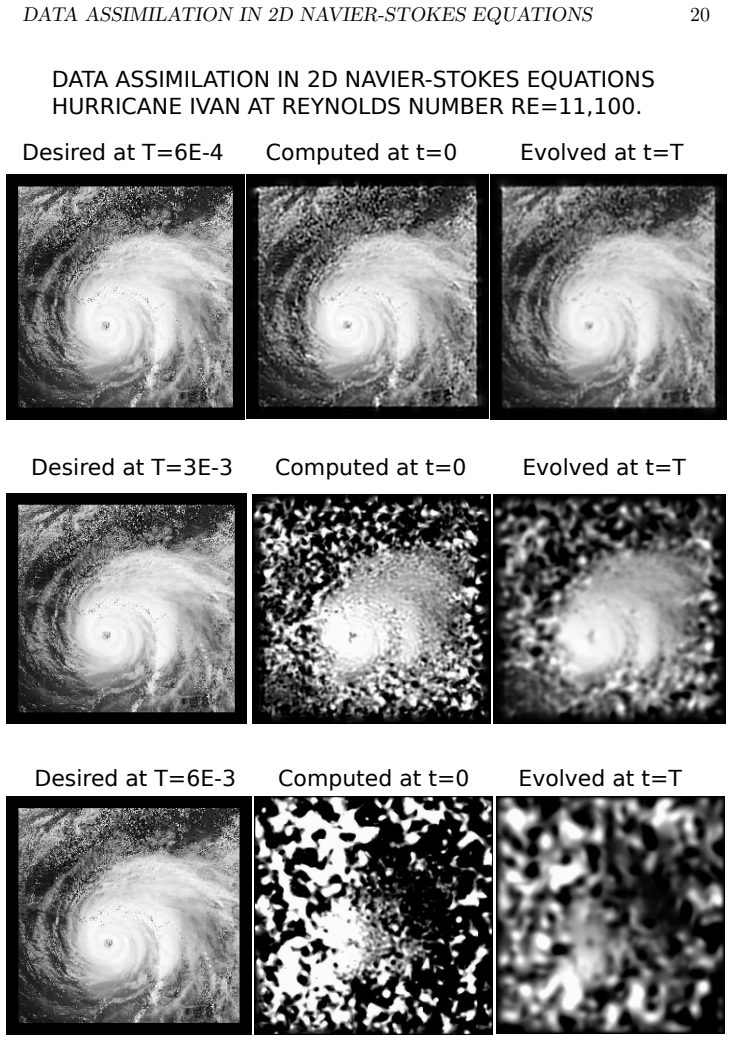
On the paper's own terms, the discovery is that the ill-posed backward-in-time Navier-Stokes initial value problem—locate initial $\psi,u,v,\omega$ at $t=0$ whose forward evolution reproduces given hypothetical data at $t=T$—is practically solvable for non-smooth image-like data by a stabilized explicit $\mathcal{O}(\Delta t)^2$ leapfrog scheme, even when the data are not an actual solution at time $T$ and even when $T$ is many orders of magnitude beyond the conservative logarithmic-convexity bound. The central numerical evidence is the Hurricane Ivan example: with $\nu=0.01$, Reynolds number about $11{,}100$, and extremely non-smooth stream-function data, assimilation was successful from $T$ on the order of $10^{-4}$, while the convexity estimates following Eq. (12) indicated $T$ would need to be on the order of $10^{-9}$. The paper explains the discrepancy by noting that worst-case uncertainty estimates must anticipate the worst possible error accumulation, which individual data sets do not necessarily realize. Theorems 1 and 2 give stability and error bounds for a related linear constant-coefficient problem, showing that the stabilizing operator $S$ keeps the leapfrog march stable and that the error is governed by $\delta \exp(4n|\Delta t|\lambda_J)$ plus a stabilization penalty of order $(\lambda_J)^{-p}$. The paper does not prove nonlinear stability; it states that linear stability is necessary but not sufficient and relies on the empirically chosen RAW filter to control leapfrog nonlinear instability.
Load-bearing premise
The load-bearing premise is that the linear constant-coefficient stability analysis, together with the empirically tuned RAW filter, keeps the backward march stable for the full nonlinear Navier-Stokes equations at the target $T$; the paper itself states that linear stability is necessary but not sufficient in nonlinear leapfrog computations, and no nonlinear stability proof is provided.
Editorial extensions
If this is right
- Data assimilation for 2D Navier-Stokes flows at high Reynolds number can be attacked by direct explicit backward marching, avoiding the cost of neural-network training or iterative variational methods.
- Successful assimilation times can exceed the logarithmic-convexity bound by orders of magnitude in individual cases, because worst-case estimates are not realized by specific non-smooth data sets.
- The same scheme will not succeed for arbitrarily large T; the paper shows degradation at larger T and stresses that unsuccessful assimilation is possible.
- Backward-stabilized leapfrog computations can serve as an independent check on machine-learning-based data assimilation and on suspected hallucinations in such computations.
Reading between the lines
- Editorial inference: If the empirical T-horizon observed here holds for other non-smooth data, the practical limitation on backward data assimilation in dissipative geophysical flows may be set by data smoothness and by the onset of nonlinear leapfrog instability, rather than by the exponential worst-case convexity bounds.
- Editorial inference: A testable extension is to measure how the reconstruction error at fixed $T$ scales with data noise $\delta$ in the Hurricane Ivan example; the linear theory predicts essentially linear growth through the factor $\exp(4\lambda_J T)$, and the paper's data do not directly resolve that scaling.
- Editorial inference: The same stabilized backward leapfrog with a Fourier smoothing operator could be applied to other dissipative image-based assimilation problems, such as heat or advection-diffusion equations, since the stabilizing mechanism only depends on the Laplacian spectrum through $\lambda_J$.
- Editorial inference: The smoothing penalty visible in the tables, where evolved derivative norms fall well below the desired data, suggests a practical strategy: accept mildly smoothed reconstructions and use the backward solution as a regularized prior rather than as an exact initial condition.
Editorial analysis
A structured set of objections, weighed in public.
Referee Report
Summary. The paper proposes a stabilized explicit leapfrog finite difference scheme, run backward in time, for data assimilation in the 2D incompressible Navier-Stokes equations. Given hypothetical, possibly non-smooth data at time T, the scheme computes initial data at t=0 that are then evolved forward to approximate the given data. The stability analysis is restricted to a linear constant-coefficient problem and the central theorems are stated without proof, deferred to the author's prior paper [30]. Nonlinear leapfrog instability is addressed by adding a Robert-Asselin-Williams filter. The paper reports successful assimilation for several satellite and chart images at T values allegedly several orders of magnitude larger than Knops-Payne uncertainty estimates suggest, alongside unsuccessful examples.
Significance. If the method were shown to be reliable, it would offer a cheap explicit alternative to iterative and machine-learning data assimilation for ill-posed backward Navier-Stokes problems. The paper includes an honest discussion of limitations, explicitly concedes that linear stability is not sufficient for the nonlinear scheme, and acknowledges that success is assessed visually. However, the support for the central claim is weakened by the absence of proved nonlinear stability, the reliance on interactively tuned parameters, and an apples-to-oranges comparison with the Knops-Payne bounds. The paper is a useful contribution to the debate on explicit stabilized backward marching, but it does not yet provide convincing evidence for the headline claim.
major comments (4)
- [Section 5, Theorems 1 and 2, Eqs. (46), (51)] The two theorems that underpin the entire error analysis are stated without proof and deferred to the author's prior paper [30], despite the abstract claiming the paper is self-contained. The data assimilation error bounds in Eqs. (54)-(56) rely on these theorems. For a journal submission, either the proofs should be included or the paper should explicitly state that its theoretical foundation is entirely contained in [30] and explain why the results transfer verbatim to the present setting.
- [Section 6, nonlinear stability transfer] The paper acknowledges that linear stability is necessary but not sufficient for nonlinear leapfrog computations, and that a RAW filter must be added to prevent nonlinear instability. However, no nonlinear stability analysis or numerical convergence study is provided for the stabilized backward scheme applied to the full Navier-Stokes equations. Since all reported experiments are nonlinear, the linear error bounds in Section 5 do not directly apply to them. This gap is load-bearing because the paper's central claim of successful data assimilation rests on the empirical behavior of the nonlinear scheme.
- [Section 7, Tables 2-5] The success metric is inadequate. The tables report separate L2 norms of the desired and evolved fields, not errors between them, and the evolved vorticity norms are 25-75% below the desired norms (e.g., Table 4: 4426 vs 18094; Table 2: 3951 vs 14301). The paper itself notes in the text around Figure 6 that the evolved data are noticeably smoother than the hypothetical data. A field whose vorticity is reduced by 70-75% is not self-evidently a useful approximation for data assimilation, especially if gradients or derived quantities are of interest. The authors should report quantitative error measures, such as relative L2 errors for u, v, and omega, and ideally pointwise or structural similarity metrics.
- [Section 7 vs. Section 3, Eq. (12)] The claimed discrepancy of five orders of magnitude between the achievable T (about 10^-4) and the Knops-Payne estimate (about 10^-9) is not substantiated because the constants E and Q in Eq. (12) are evaluated on the raw, non-smooth hypothetical data (Umax about 111, sup|omega| about 1.5e5). The actual computed backward/forward solution is smooth and has much smaller sup norms. Since a, b, c, and Gamma(t) in Eq. (8) depend exponentially on these constants, re-evaluating E and Q on the computed solution could change the estimate by many orders of magnitude. Moreover, Eq. (48) assumes the given data approximate a true Navier-Stokes solution at time T, which is not verified for arbitrary images. The comparison in Section 7 should be recomputed on the actual computed solution, or the authors should explicitly state that the comparison is against the raw data and not against the reconstructed smooth solution.
minor comments (4)
- [Abstract and throughout] Numerous typos and spacing errors distract from the presentation, including 'sc heme' in the abstract, 'unconditonally' and 'instabilty' in Sections 4 and 6, and 'apropriate' repeated in Section 1.
- [Section 5, Eq. (12)] The constants E and Q in Eqs. (6) and (7) are not defined explicitly as functions of the given data; Eq. (12) states E^2 > U_max^2 but does not specify how E is chosen. A precise definition would improve reproducibility of the estimates.
- [Section 7, figures and tables] The figure captions do not list the numerical parameters used for each experiment (gamma, p, eta, Delta t, and the exact final T for each row). Without these parameters, the experiments are not reproducible from the manuscript alone.
- [Section 4, Eq. (21)] The indexing of the leapfrog scheme is confusing: Eq. (20) defines theta^1 and omega^1, while Eq. (21) uses n=1,2,...,N with theta^{n+1}=S omega^n and omega^{n+1}=S theta^n + 2 Delta t S L^dagger omega^n. It would be clearer to state explicitly how the first step is handled and how the filter in Eq. (59) modifies the first two steps.
Circularity Check
Partial circularity: the stability/error analysis is imported from the author's own prior paper, and the headline success at T~1e-4 is obtained by interactive parameter tuning plus visually selected first rows, so the claimed contrast with Eq. (12) is not an independent prediction.
-
self citation load bearing
[Section 5, Lemmas 1-2 and Theorems 1-2, Eqs. (40)-(52)]
"Below, Lemmas 1 and 2, along with Theorems 1 and 2, are stated without proof. Using identical notation, proofs of these results may be found in [30]. ... Proof : See [30, Lemma 5.1] ... Proof : See [30, Theorem 5.2]."
The central theoretical support for the stabilized backward leapfrog scheme, namely the error bounds in Theorem 2 that are later used in Eqs. (54)-(56) to justify successful data assimilation, is not derived in this paper. It is cited from the author's own previous paper [30], which is not reproduced, machine-checked, or independently validated here. This is load-bearing because Lemma 1 and Theorem 2 are the only quantitative stability/error analysis offered for the scheme; if [30] itself merely asserts the same ansatz, the derivation chain closes without new mathematical content.
-
fitted input called prediction
[Section 6, Remark 3; Section 7, Figures 2-5 and Tables 2-5]
"interactive adjustment of the parameter pair (gamma,p) in Eqs. (18,19) ... often leads to useful reconstructions. ... The values of (gamma,p) are increased slowly if instability is detected, and are likewise decreased slowly to increase sharpness, provided no instability results. As is the case with binoculars, useful results are generally obtained after relatively few trials. There may be several possible good solutions."
The reported successes are not predictions from a fixed, blind algorithm: the smoothing parameters (gamma,p) are interactively tuned until an acceptable reconstruction appears, and the first rows of Figures 2-5 are 'considered a successful example' while success is judged visually. The claimed result that T~1e-4 works despite the Eq. (12) estimate of T~1e-9 is therefore a fitted outcome rather than an independent test. The parameter choice is adapted to the displayed images, so the demonstration does not quantify the predictive power of the stabilized scheme at large T.
1 more flagged steps
-
other
[Section 7, Hurricane Ivan discussion and Table 4; Section 3, Eq. (12)]
"successful assimilation from a T value on the order of 10^{-4}, was found possible in the Hurricane Ivan image, given the uncertainty estimates following Eq. (12) in Section 3. These estimates indicated a necessary value for T on the order of 10^{-9}. ... the evolved image at time T is a computed solution to the 2D Navier-Stokes equations. Such a solution would necessarily be a smooth approximation to hypothetical data that might be far from an actual solution at the same time T>0."
The uncertainty constants in Eq. (12) are evaluated from the raw non-smooth image class, with Umax about 111, sup|omega| about 1.5e5, leading to E^2>12400, Q^2>2.19e10 and hence a,b,c values many orders of magnitude larger than for the evolved solution. The paper's 'successful' evolved image is smooth: Table 4 gives evolved vorticity norm 4426 versus desired 18094 and velocity norms about 30-40% lower. Thus the claimed five-orders-of-magnitude discrepancy compares the Eq. (12) bound for the raw data class with a computed smooth solution that does not satisfy the same E,Q class. The asserted contrast is therefore not a valid measurement of the scheme's performance against the theoretical bound; it is an equivocation between two different mathematical objects.
full rationale
The paper contains real computational experiments, and the stabilized backward leapfrog idea has independent content beyond a pure tautology. However, the strongest advertised conclusion, that assimilation succeeds at T values five orders of magnitude beyond the Knops-Payne uncertainty bound, is not a self-contained derivation. Three factors reduce the weight of that claim. First, the only theoretical error bounds for the scheme are stated without proof and deferred to the author's own prior paper [30], making the central stability premise a self-citation rather than an argument presented here. Second, the successful examples rely on interactive choice of the smoothing parameters (gamma,p) and on preselected first-row images judged visually, so the outcome is fitted rather than predicted. Third, the comparison with Eq. (12) is not apples-to-apples: the bound is computed from the raw image's extreme sup norms, while the evolved solution is smooth and has substantially smaller norms, as the tables show. None of these points individually makes the paper definitionally circular, but together they mean that the headline 'orders of magnitude beyond the uncertainty estimates' reduces substantially to tuning plus a mismatched comparison. A score of 6 reflects partial circularity: the empirical successes are real demonstrations of the scheme with chosen parameters, but they do not provide an independent prediction at the claimed T values.
Assumptions & free parameters
free parameters (3)
- gamma (smoothing operator parameter) =
not reported per example; stated range 10^-14 to 10^-7
- p (smoothing operator exponent) =
not reported per example; stated range 2.5 to 3.5
- eta (RAW filter coefficient) =
not reported per example; stated range 0.01 to 0.2
assumptions (2)
- ad hoc to paper The linear constant-coefficient stability analysis (Theorems 1-2, proved in [30]) extends to the full nonlinear Navier-Stokes scheme when combined with the RAW filter.
- domain assumption The rescaled 256x256 image intensity arrays define valid stream functions satisfying the homogeneous boundary conditions in Eq. (1).
Cite this review
Pith. "Pith review of Data assimilation in 2D incompressible Navier-Stokes equations, using a stabilized explicit $O(\Delta t)^2$ leapfrog finite difference scheme run backward in time." pith.science (2026). https://pith.science/paper/FCMK25OD
@misc{pith2026241114617,
  author       = {Pith},
  title        = {Pith review of: Data assimilation in 2D incompressible Navier-Stokes equations, using a stabilized explicit $O(\Delta t)^2$ leapfrog finite difference scheme run backward in time},
  year         = {2026},
  howpublished = {\url{https://pith.science/paper/FCMK25OD}},
  note         = {Machine review of arXiv:2411.14617}
}
abstract
For the 2D incompressible Navier-Stokes equations, with given hypothetical non smooth data at time $T > 0 $that may not correspond to an actual solution at time $T$, a previously developed stabilized backward marching explicit leapfrog finite difference scheme is applied to these data, to find initial values at time $t = 0$ that can evolve into useful approximations to the given data at time $T$. That may not always be possible. Similar data assimilation problems, involving other dissipative systems, are of considerable interest in the geophysical sciences, and are commonly solved using computationally intensive methods based on neural networks informed by machine learning. Successful solution of ill-posed time-reversed Navier-Stokes equations is limited by uncertainty estimates, based on logarithmic convexity, that place limits on the value of $T > 0$. In computational experiments involving satellite images of hurricanes and other meteorological phenomena, the present method is shown to produce successful solutions at values of $T > 0$, that are several orders of magnitude larger than would be expected, based on the best-known uncertainty estimates. However, unsuccessful examples are also given. The present self-contained paper outlines the stabilizing technique, based on applying a compensating smoothing operator at each time step, and stresses the important differences between data assimilation, and backward recovery, in ill-posed time reversed problems for dissipative equations. While theorems are stated without proof, the reader is referred to a previous paper, on Navier-Stokes backward recovery, where these proofs can be found.
Figures


Figures from the paper (3 more)


Reference graph
Works this paper leans on
-
[30]
Carasso AS. Stabilized leapfrog scheme run backward in time, and the explicit O(∆ t)2 stepwise computation of ill-posed time- reversed 2D Navier-Stokes equations. Inverse Probl. Sci. Eng. 2 021; DOI:10.1080/17415977.2021.1972997
arXiv 2021
-
[1]
Tracking the model: data a s- similation by artificial neural network
Cintra R, de Campos Velho HF, Cocke S. Tracking the model: data a s- similation by artificial neural network. 2016 International Joint Co nfer- ence on Neural Networks (IJCNN), Vancouver, BC, Canada. 201 6:403-410. DOI:10.1109/IJCNN.2016.7727227
arXiv 2016
-
[2]
A machine learning aug- mented data assimilation method for high resolution observations
Howard LJ, Subramanian A, Hoteit I. A machine learning aug- mented data assimilation method for high resolution observations. J our- nal of Advances in Modeling Earth Systems. 2024;16,e2023MS00377 4. https://doi.org/10.1029/2023MS003774
-
[3]
Data Assimilation for Geo- physical Fluids
Blum J, Le Dimet F-X, Navon I-M. Data Assimilation for Geo- physical Fluids. Handbook of Numerical Analysis. 2009;14:385-441. https://doi.org/10.1016/S1570-8659(08)00209-3
-
[4]
He Q, Barajas-Solano D, Tartakovsky G, et al. Physics-informe d neural networks for multiphysics data assimilation with applica- tion to subsurface transport. Advances in Water Resources 202 0; https://doi.org/10.1016/j.advwatres.2020.103610
-
[5]
Deep data assimilation: integrat- ing deep learning with data assimilation
Arcucci R, Zhu J, Hu S, et al. Deep data assimilation: integrat- ing deep learning with data assimilation. Appl. Sci. 2021;11:1114. https://doi.org/10.3390/app11031114
-
[6]
Data assimilation with deep neural nets in- formed by nudging
Antil H, Lohner R, Price R. Data assimilation with deep neural nets in- formed by nudging. https://arxiv.org/abs/2111.11505. Novembe r 2021
arXiv 2021
-
[7]
A novel neural network training fra mework with data assimilation
Chen C, Dou Y, Chen J, et al. A novel neural network training fra mework with data assimilation. Journal of Supercomputing. 2022;78:19020– 19045. https://doi.org/10.1007/s11227-04629-7
Show all 46 references
-
[8]
Iterative methods for data a ssimilation for Burgers’ equation
Lundvall J, Kozlov V, Weinerfelt P. Iterative methods for data a ssimilation for Burgers’ equation. J. Inverse Ill-Posed Probl. 2006;14:505–5 35
2006
-
[9]
A nudging-based data assimilation method for oceanographuc problems: the back and forth nudging (BFN) algor ithm
Auroux D, Blum J. A nudging-based data assimilation method for oceanographuc problems: the back and forth nudging (BFN) algor ithm. Proc. Geophys. 2008;15:305–319
2008
-
[10]
Unsteady adjoint method for the optimal con trol of ad- vection and Burgers’ equation using high order spectral differenc e method
Ou K, Jameson A. Unsteady adjoint method for the optimal con trol of ad- vection and Burgers’ equation using high order spectral differenc e method. 49th AIAA Aerospace Science Meeting, 4-7 January 2011. Orlando , Florida
2011
-
[11]
The back and forth nudging algorithm for da ta assimi- lation problems: theoretical results on transport equations
Auroux D, Nodet M. The back and forth nudging algorithm for da ta assimi- lation problems: theoretical results on transport equations. ESA IM:COCV 2012;18:318–342
2012
-
[12]
An evolution of the back and forth nudg- ing for geophysical data assimilation: application to Burgers equatio n and comparison
Auroux D, Bansart P, Blum J. An evolution of the back and forth nudg- ing for geophysical data assimilation: application to Burgers equatio n and comparison. Inverse Probl. Sci. Eng. 2013;21:399-419 DATA ASSIMILATION IN 2D NA VIER-STOKES EQUATIONS 25
2013
-
[13]
Numerical aspects of large-tim e optimal control of Burgers’ equation
Allahverdi N, Pozo A, Zuazua E. Numerical aspects of large-tim e optimal control of Burgers’ equation. ESAIM Mathematical Modeling and N umer- ical Analysis 2016;50:1371–1401
2016
-
[14]
Filtered gradient algorithms for inverse des ign problems of one-dimensional Burgers’ equation
Gosse L, Zuazua E. Filtered gradient algorithms for inverse des ign problems of one-dimensional Burgers’ equation. Innovative Algorithms and Analysis 2017;197–227
2017
-
[15]
Special issue on in- verse problems in geosciences
de Campos Velho HF, Barbosa VCF, Cocke S. Special issue on in- verse problems in geosciences. Inverse Probl. Sci. Eng. 2013;21:35 5-356. DOI:10.1080/17415977.2012.712532
2013
-
[16]
Contaminant source identification in ac- quifers: a critical view
Gomez-Hernandez JJ, Xu T. Contaminant source identification in ac- quifers: a critical view. Math Geosci 2022;54:437–458
2022
-
[17]
Non-point contamin ant source identification in an acquifer using the ensemble smoother with multiple d ata assimilation
Xu T, Zhang W, Gomez-Hernandez JJ, et al. Non-point contamin ant source identification in an acquifer using the ensemble smoother with multiple d ata assimilation. Journal of Hydrology 2022; 606:127405
2022
-
[18]
Properties of advection algo rithms in the context of variational data assimilation
Vukicevic T, Steyskal M, Hecht M. Properties of advection algo rithms in the context of variational data assimilation. Monthly Weather Rev iew 2001;129:1221–1231
2001
-
[20]
Data assimilation in 2D nonlinear advection diffusion eq ua- tions, using an explicit stabilized leapfrog scheme run backwrd in time
Carasso AS. Data assimilation in 2D nonlinear advection diffusion eq ua- tions, using an explicit stabilized leapfrog scheme run backwrd in time. NIST Technical Note 2227, July 12 2022. DOI:10.6028/NIST.TN2227
2022 doi
-
[21]
Data assimilation in 2D hyperbolic/parabolic systems us- ing a stabilized explicit finite difference scheme run backward in time
Carasso AS. Data assimilation in 2D hyperbolic/parabolic systems us- ing a stabilized explicit finite difference scheme run backward in time. Applied Mathematics in Science and Engineering, 2024;32:1,228641. DOI:10.1080/27690911.2023.228641
2024 arXiv
-
[22]
Difference Methods for Initial Value P roblems
Richtmyer RD, Morton KW. Difference Methods for Initial Value P roblems. 2nd ed. New York (NY): Wiley; 1967
1967
-
[23]
Compensating operators and stable backward in t ime march- ing in nonlinear parabolic equations
Carasso AS. Compensating operators and stable backward in t ime march- ing in nonlinear parabolic equations. Int J Geomath 2014;5:1–16
2014
-
[24]
Stable explicit time-marching in well-posed or ill-posed non- linear parabolic equations
Carasso AS. Stable explicit time-marching in well-posed or ill-posed non- linear parabolic equations. Inverse Probl. Sci. Eng. 2016;24:1364–1 384
2016
-
[25]
Stable explicit marching scheme in ill-posed time-reve rsed vis- cous wave equations
Carasso AS. Stable explicit marching scheme in ill-posed time-reve rsed vis- cous wave equations. Inverse Probl. Sci. Eng. 2016;24:1454–1474
2016
-
[26]
Stabilized Richardson leapfrog scheme in explicit ste pwise computation of forward or backward nonlinear parabolic equations
Carasso AS. Stabilized Richardson leapfrog scheme in explicit ste pwise computation of forward or backward nonlinear parabolic equations . Inverse Probl. Sci. Eng. 2017;25:1–24. DATA ASSIMILATION IN 2D NA VIER-STOKES EQUATIONS 26
2017
-
[28]
Stable explicit stepwise marching scheme in ill- posed t ime- reversed 2D Burgers’ equation
Carasso AS. Stable explicit stepwise marching scheme in ill- posed t ime- reversed 2D Burgers’ equation. Inverse Probl. Sci. Eng. 2018;27 (12):1-17. DOI:10.1080/17415977.2018.1523905
2018
-
[29]
Computing ill-posed time-reversed 2D Navier-Stok es equa- tions, using a stabilized explicit finite difference scheme marching back ward in time
Carasso AS. Computing ill-posed time-reversed 2D Navier-Stok es equa- tions, using a stabilized explicit finite difference scheme marching back ward in time. Inverse Probl. Sci. Eng. 2019; DOI:10.1080/17415977.2019 .1698564
2019
-
[31]
Finite difference schemes for incompressible flow based on local pressure boundary conditions
Johnston H, Liu JG. Finite difference schemes for incompressible flow based on local pressure boundary conditions. J. Comput. Phys. 2002;18 0:120–154
2002
-
[32]
Solution of 2D Navier-Stokes equat ion by cou- pled finite difference-dual reciprocity boundary element method
Ghadimi P, Dashtimanesh A. Solution of 2D Navier-Stokes equat ion by cou- pled finite difference-dual reciprocity boundary element method. A pplied Mathematical Modelling 2011;35:2110–2121
2011
-
[33]
Non-Standard and Improperly Posed P roblems
Ames KA, Straughan B. Non-Standard and Improperly Posed P roblems. New York (NY): Academic Press; 1997
1997
-
[34]
Some remarks on ill-posed problems for viscous fluids
Payne LE. Some remarks on ill-posed problems for viscous fluids. Int. J. Engng Sci. 1992;30:1341–1347
1992
-
[35]
Logarithmic convexity and other techniques applied t o prob- lems in continuum mechanics
Knops RJ. Logarithmic convexity and other techniques applied t o prob- lems in continuum mechanics. In: Knops RJ, editor. Symposium on non - well-posed problems and logarithmic convexity. Vol. 316, Lecture no tes in mathematics. New York (NY): Springer-Verlag; 1973
1973
-
[36]
On the stability of solutions of the Navier-S tokes equations backward in time
Knops RJ, Payne LE. On the stability of solutions of the Navier-S tokes equations backward in time. Arch. Rat. Mech. Anal. 1968;29:331–33 5
1968
-
[37]
Uniqueness and continuous dependence criteria for the Navier- Stokes equations
Payne LE. Uniqueness and continuous dependence criteria for the Navier- Stokes equations. Rocky Mountain J. Math. 1971;2:641–660
1971
-
[38]
Reconstructing the past from imprecise knowledg e of the present: Effective non-uniqueness in solving parabolic equations ba ckward in time
Carasso AS. Reconstructing the past from imprecise knowledg e of the present: Effective non-uniqueness in solving parabolic equations ba ckward in time. Math. Methods Appl. Sci. 2012;36:249-–261
2012
-
[39]
Computing small solutions of Burgers’ equation bac kwards in time
Carasso A. Computing small solutions of Burgers’ equation bac kwards in time. J. Math. Anal. App. 1977;59:169–209
1977
-
[40]
Stability estimates for Burger s-type equations backward in time
H` ao DN, Nguyen VD, Nguyen VT. Stability estimates for Burger s-type equations backward in time. J. Inverse Ill Posed Probl. 2015;23:41– 49. DATA ASSIMILATION IN 2D NA VIER-STOKES EQUATIONS 27
2015
-
[41]
An example of non-linear computational instability
Phillips NA. An example of non-linear computational instability. In: Bolin B. editor, The Atmosphere and the Sea in Motion. Rockefeller Instit ute; New York (NY) 1959. p. 501-504
1959
-
[42]
On the instability of Leapfrog and Crank-Nicolson a pproxima- tions of a nonlinear partial differential equation
Fornberg B. On the instability of Leapfrog and Crank-Nicolson a pproxima- tions of a nonlinear partial differential equation. Math Comput. 197 3;27:45- 57
-
[43]
Studies in numerical nonlinear instability I
Sanz-Serna JM. Studies in numerical nonlinear instability I. Why d o leapfrog schemes go unstable ? SIAM J. Sci. Stat. Comput. 1985;6:9 23- 938
1985
-
[44]
Frequency filter for time integrations
Asselin R. Frequency filter for time integrations. Mon Weather R ev. 1972;100:487-490
1972
-
[45]
A proposed modification to the Robert-Asselin time filte r
Williams PD. A proposed modification to the Robert-Asselin time filte r. Mon Weather Rev. 2009;137:2538-2546
2009
-
[46]
The RA W filter: An improvement to the Robert-Asselin fi lter in semi-implicit integrations
Williams PD. The RA W filter: An improvement to the Robert-Asselin fi lter in semi-implicit integrations. Mon Weather Rev. 2011;139:1996-2007
2011
-
[47]
The effects of the RA W filter on th e climatology and forecast skill of the SPEEDY model
Amezcua J, Kalnay E, Williams PD. The effects of the RA W filter on th e climatology and forecast skill of the SPEEDY model. Mon Weather Rev . 2011;139:608-619
2011
-
[48]
Stability analysis of the Crank-Nico lson- Leapfrog method with the Robert-Asselin-Williams time filter
Hurl N, Layton W, Li Y, et al. Stability analysis of the Crank-Nico lson- Leapfrog method with the Robert-Asselin-Williams time filter. BIT Num er Math. 2014;54:1009-1021
2014
Reviewed August 12, 2026 · model on record in the stance chip above.
Discussion (0). Continue with ORCID to comment.