REVIEW 3 major objections 6 minor 38 references
Why is My Route Different Today? An Algorithm for Explaining Route Selection
T0 review · 3 major / 6 minor · reviewed 2026-08-07 · deepseek-v4-flash
Pith's one-line read This paper proposes that a route change can be explained by a small set of traffic-laden road segments, found as the optimum of a linear program and computed by a flow-based combinatorial algorithm.
desk verdict The SVE formalization is clean and the experiments are suggestive, but the missing termination proof for the residual augmentation loop keeps the main efficiency claim from being established. read the letter →
The pith
A machine-rendered reading of the paper's core claim, the machinery that carries it, and where it could break.
The reading
What carries the argument
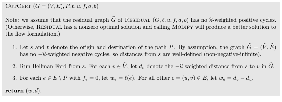
The load-bearing object is the cut-formulation LP1: minimize $\sum_{e\in E(G)} \tau(e)(w_e-\ell(e))$ over weights $w_e$ and distance potentials $d_v$, subject to $\ell(e)\le w_e\le u(e)$ on every arc, $d_v-d_u\le w_e$ on every arc, and $d_v-d_u=w_e$ on arcs of the path $P$. Its optimum is a $\tau$-simple valid explanation. The algorithm does not call an LP solver: it forms the flow-formulation dual, builds a residual graph whose arcs carry $\hat\kappa$ weights, and repeatedly finds positive-$\hat\kappa$ cycles and applies Modify to improve the dual solution. When no positive cycle remains, CutCert runs Bellman-Ford on the residual graph and constructs primal weights $w_e=d_v-d_u$, producing a zero-duality-gap pair that certifies optimality. That cycle-augmenting mechanism is what lets the method scale to graphs with tens of millions of arcs.
What would settle it
Instrument the appendix's residual augmenting loop on the published road graphs, or on small directed graphs built to admit adversarial cycle choices, and count the Modify calls: a single instance whose iteration count grows faster than polynomially with the number of arcs, or a run that never terminates, would refute the algorithm's efficiency claim.
Extended reading notes
Core claim
On the paper's own terms, the discovery is that the question 'which traffic conditions caused this route?' has a tractable optimal answer. For a returned path P, an explanation is a weight vector w that keeps every arc between its free-flow travel time $\ell(e)$ and its current traffic time $u(e)$, keeps P a shortest s-t path, and minimizes the $\tau$-valuation $\sum_{e\in E(G)} \tau(e)(w_e-\ell(e))$; such a w is the paper's $\tau$-simple valid explanation. The paper proves that this program's LP optimum always satisfies the sufficiency and validity conditions, gives a dual flow formulation whose residual graph lets a cycle-augmenting algorithm drive the duality gap to zero, and shows theoretically that in closure scenarios the SVE's support is contained in the penalty-based explanation's support. Experiments report that SVE support stays within the true closed segments in nearly all valid query pairs and uses a median of roughly ten percent of the incident path arcs.
Load-bearing premise
The efficiency claim hangs on the assumption that repeatedly finding positive-weight cycles in the residual graph and updating the dual solution eventually terminates after few iterations; the appendix shows each step improves the objective locally but never states a bound on the number of iterations or a rule for choosing cycles.
Editorial extensions
If this is right
- In single-closure scenarios, an SVE never needs arcs outside the original no-traffic shortest path, and for the paper's three $\tau$ choices its support is contained in the penalty-based explanation's support.
- For multiple closures with $\tau(e)=1/(u(e)-\ell(e))$, SVE support is always a subset of PBE support, so the relaxation matches the best-known baseline in the exact setting where the baseline is well behaved.
- When every road segment is pliable, the advantage shifts decisively: SVEs stay within the true closed segments in 93-100 percent of valid query pairs while PBEs never do.
- In delay ('incident') scenarios, SVEs keep at least 83 percent of the relevant penalized arcs while using a median of about 10 percent of the number of arcs in the penalized path set.
- A subgraph-restricted variant answers a query in about 50 milliseconds on a laptop-class chip, putting the explainer in the range of real-time navigation use.
Reading between the lines
- The exact minimum-cardinality explanation is NP-hard, so SVE optimality is only optimality within the LP relaxation; an obvious test is to compare SVE support to the true integer-programming optimum on small instances to see how much the relaxation costs.
- The same cut/flow template should transfer to other route objectives—scenic, safe, or fuel-minimizing—by swapping the lower and upper weight functions, as long as the route to explain is still a shortest path under the modified weights.
- The runtime claim depends on the unstated termination of the residual cycle-augmentation loop; a polynomial iteration count or a concrete cycle-selection rule would convert the empirical speed into a guarantee.
- Experimental closures are chosen by an arterial-road heuristic, so the near-perfect recovery of closed segments may be partly a property of the test design; uniformly random closures would be a stricter check.
Editorial analysis
A structured set of objections, weighed in public.
Referee Report
Summary. The paper introduces simple valid explanations (SVEs) for route recommendations. Given a digraph with free-flow arc weights ℓ and traffic-aware weights u, and a reported shortest s-t path P under u, an SVE is a weight vector w with ℓ(e) ≤ w(e) ≤ u(e) under which P remains an s-t shortest path, chosen to minimize the τ-valuation Σ τ(e)(w(e) − ℓ(e)); this is LP1. Theorem 2.1 shows that LP1 optima are exactly the τ-simple valid explanations. Section 2 claims a novel flow-based combinatorial solver for LP1 on graphs with hundreds of millions of arcs, and Appendix A develops residual graphs, an augmenting routine Modify, and a certificate routine CutCert. Sections 3–5 provide structural results (Theorems 3.1 and 3.2) comparing SVE support to penalty-based explanations (PBEs) in closure scenarios, and experiments on Baden-Württemberg and Washington road networks reporting SVE support sizes and containment rates.
Significance. If the algorithmic claim were established, this would be a useful and timely contribution: the LP relaxation of an NP-hard explanation problem is clean and well-motivated, the duality-gap certificate approach is elegant, and Theorems 3.1 and 3.2 are genuine structural results that are not merely fitted to the data. The experiments are on realistic large-scale road networks with released code, and the scenarios are constructed to recover planted causes, which is an honest evaluation protocol. The main gap is that the alleged efficient algorithm is not delivered: the convergence of the augmenting loop in Appendix A is unproven, and the residual-graph construction is ambiguous on antiparallel arcs. Because the efficiency claim is the paper's headline, the contribution is not yet fully substantiated; nonetheless, the theoretical framework and the structural theorems are valuable, and the gaps appear localizable.
major comments (3)
- [Appendix A; Sections 2.1–2.2] The manuscript's central claim is that LP1 can be solved efficiently by the flow-based algorithm, but Appendix A never closes the loop. Claims A.2 and A.3 prove local statements — a feasible nondegenerate residual flow strictly improves the dual objective, and a residual graph with no positive bκ-weighted cycle leads to an optimal primal-dual pair via CutCert — yet no theorem states that the process 'find a positive bκ-cycle, apply Modify, repeat' terminates, and no bound is given on the number of iterations. No cycle-selection rule is specified, and no potential function is exhibited. With integral data, each Modify step increases the dual objective by at least 1, but the initial gap to optimality can be exponential in the input encoding; with rational data the increments can shrink, so even termination is not immediate. The remark in Section 2.2 that runtime is 'empirically linear in τ_max' is an experimental observation, not a guarantee. Because the abstract and Section 2.1 promise 'an efficient algorithm' for continent-scale graphs, this missing convergence theorem is load-bearing: as written, the paper establishes correct local optimality certificates but not an efficient algorithm.
- [Appendix A, Figures 7–8] The residual graph bE is defined as the set E ∪ bEres ∪ bEP of ordered pairs. Road networks typically contain antiparallel arcs, so an ordered pair (v,u) can simultaneously be an original arc in E and a reverse-residual arc in bEres (when f_{(u,v)} > 0), and similarly with bEP for arcs of P. In that case, steps 4(a)–4(c) of Residual add the same element to F, then to bFres, then to bFP in turn, moving it between the three sets as bκ(e) is recomputed by max; the final classification depends on the order of the branches. The note in Modify that 'F, bFres, and bFP form a partition of bE by definition' is therefore not justified, and the residual problem with a single merged copy of a forward arc and its reverse residual is not the intended circulation model. Claims A.2 and A.3 are not established for graphs with antiparallel arcs, which includes the experimental road networks. The construction should use distinct copies (a multiset) or explicitly justify that the merge preserves the residual objective.
- [Definition 1.1; Section 5.4, Table 3] The simplicity objective is a continuous surrogate for the number of modified arcs, so τ-optimality does not by itself bound support(w): a solution that spreads tiny increases over many arcs can have arbitrarily small valuation and large support. The support-containment theorems (Theorems 3.1 and 3.2) cover only closure scenarios under specific τ assumptions; for incident scenarios, the claim that SVEs are 'small' rests entirely on the empirical support ratios in Table 3. The paper should state this explicitly and, ideally, report how often w(e) lies strictly between ℓ(e) and u(e), since a fractional optimum weakens the interpretation of support size as the explanation size.
minor comments (6)
- [Section 2.2, Option 2] The entries of τ are required to be integral 'by rounding,' but the rounding direction is unspecified; for arcs with u(e) − ℓ(e) > 1, rounding to the nearest integer gives τ(e) = 0, which would make delays on those arcs free in the objective and would violate the positive-τ assumption of Theorem 3.2. Please specify the rounding convention and its effect.
- [Section 5.2] The text says that Theorems 3.1 and 3.2 'would show that this fraction is 1' but that the conditions fail 'due to a noncompliant choice of τ.' The experimental protocol also deletes multiple arcs within 5 hops of e_i (Section 3.1), so the deviation is not attributable to τ alone; the sentence should acknowledge both sources of noncompliance.
- [Tables 1 and 2] The column arrangement ('# paths ≤10 2 10' over 'SVE PBE') is hard to read; please restructure the tables, for example with separate rows for SVE and PBE or separate tables for k = 1 and k = 9.
- [Section 2.3] The subgraph on which the 50 ms runtime is measured is not described, so the real-time claim cannot be reproduced; please specify the subgraph construction and the query set.
- [Sections 2.1 and 2.2] Section 2.1 is titled 'Runtime of Solving the Cut Formulation' but contains no runtime statement; either state a formal bound or rename the section. Also, the phrase 'in the appendix of the full version of this paper' should refer to Appendix A of this manuscript.
- [Throughout] There are several typos and notational slips, e.g., 'the e i s' in Section 3.1, the footnote in Section 1.2 saying 'e does not contribute' without specifying which e, and the Figure 1 caption comparing 'the total weight of arcs' without stating that the comparison is of τ-valuation.
Circularity Check
Derivation is definition-driven and self-contained; the main gap is an unproven termination bound in Appendix A, which is a correctness issue, not circularity.
full rationale
No circular step rises to the level required by the analysis. The paper defines an SVE directly as an optimizer of LP1: the objective is the τ-valuation and constraints (4)-(6) are exactly the validity and sufficiency conditions, so Theorem 2.1 is a definitional bridge rather than a prediction derived from fitted data. No parameter is fitted to the explanations later reported. Theorems 3.1 and 3.2 are derived from LP optimality, the closure-scenario construction, and the PBE definition; they do not assume their conclusions. The experimental scenarios are planted from the same road networks, so they benchmark recovery of known planted causes; this limits external validity but is not circular, because the SVE solver receives only ℓ, u, and P and never the planted set. The choice C0=10 is fixed rather than tuned to the reported outcomes. The load-bearing concern is instead a missing proof: Appendix A shows that Modify improves a feasible dual solution and that CutCert certifies optimality when no positive bκ-cycle remains, but it never proves that the augmentation loop terminates or does so in polynomially many iterations; Section 2.2's 'empirically linear in τ_max' is an experimental observation. That is an omitted-proof and completeness risk, not a circular reduction of the paper's conclusions to its inputs.
Assumptions & free parameters
free parameters (3)
- C0 in τ Option 3 =
C0 = 10
- γ in incident scenarios =
γ = 1.1
- closure neighborhood size =
5 hops around selected arc
assumptions (4)
- standard math LP duality, min-cost circulation, Bellman-Ford, and the augmenting-paths framework are used without proof.
- domain assumption Road network is a directed graph with static arc weights; closures are infinite weights, and time-dependent traffic is not modeled.
- ad hoc to paper The iterative residual-augmentation procedure is assumed to terminate and find an optimal SVE.
- ad hoc to paper Rounding or replacing τ with Option 3 is assumed not to change explanation quality.
Cite this review
Pith. "Pith review of Why is My Route Different Today? An Algorithm for Explaining Route Selection." pith.science (2026). https://pith.science/paper/FHCFLVR3
@misc{pith2026250605604,
  author       = {Pith},
  title        = {Pith review of: Why is My Route Different Today? An Algorithm for Explaining Route Selection},
  year         = {2026},
  howpublished = {\url{https://pith.science/paper/FHCFLVR3}},
  note         = {Machine review of arXiv:2506.05604}
}
read the original abstract
Users of routing services like Apple Maps, Google Maps, and Waze frequently wonder why a given route is proposed. This question particularly arises when dynamic conditions like traffic and road closures cause unusual routes to be proposed. While many dynamic conditions may exist in a road network at any time, only a small fraction of those conditions are typically relevant to a given user's route. In this work, we introduce the concept of a simple valid explanation (SVE), which consists of a small set of traffic-laden road segments that answer the following question: Which traffic conditions cause a particular shortest traffic-aware route to differ from the shortest traffic-free route? We give an efficient algorithm for finding SVEs and show that they theoretically and experimentally lead to small and interpretable answers to the question.
Figures


Figures from the paper (6 more)


Reference graph
Works this paper leans on
-
[1]
A framework for data-driven explainability in mathematical optimization
Kevin-Martin Aigner, Marc Goerigk, Michael Hartisch, Frauke Liers, and Arthur Miehlich. A framework for data-driven explainability in mathematical optimization. InProceedings of the AAAI Conference on Artificial Intelligence, volume 38, pages 20912–20920, 2024. 17
work page 2024
-
[2]
Michael O. Ball, Bruce L. Golden, and Rakesh V. Vohra. Finding the most vital arcs in a network. Oper. Res. Lett., 8(2):73–76, 1989
work page 1989
-
[3]
Yanyan Chen, Michael G. H. Bell, and Klaus Bogenberger. Reliable pretrip multipath planning and dynamic adaptation for a centralized road navigation system.IEEE Transactions on Intelligent Trans- portation Systems, 8(1):14–20, 2007
work page 2007
-
[4]
Stephen R. Chestnut and Rico Zenklusen. Interdicting structured combinatorial optimization problems with{0,1}-objectives.Math. Oper. Res., 42(1):144–166, 2017
work page 2017
-
[5]
Explainable k-means and k- medians clustering
Sanjoy Dasgupta, Nave Frost, Michal Moshkovitz, and Cyrus Rashtchian. Explainable k-means and k- medians clustering. InProceedings of the 37th International Conference on Machine Learning, ICML’20. JMLR.org, 2020
work page 2020
-
[6]
Towards a rigorous science of interpretable machine learning.arXiv preprint arXiv:1702.08608, 2017
Finale Doshi-Velez and Been Kim. Towards a rigorous science of interpretable machine learning.arXiv preprint arXiv:1702.08608, 2017
arXiv 2017
-
[7]
Explainable ai (xai): Core ideas, techniques, and solutions.ACM Comput
Rudresh Dwivedi, Devam Dave, Het Naik, Smiti Singhal, Rana Omer, Pankesh Patel, Bin Qian, Zhenyu Wen, Tejal Shah, Graham Morgan, and Rajiv Ranjan. Explainable ai (xai): Core ideas, techniques, and solutions.ACM Comput. Surv., 55(9), January 2023
work page 2023
-
[8]
Explanations for combinatorial optimization problems.Journal of Computer Languages, 79:101272, 2024
Martin Erwig and Prashant Kumar. Explanations for combinatorial optimization problems.Journal of Computer Languages, 79:101272, 2024
work page 2024
Show all 38 references
-
[9]
Explainable data-driven optimization: from context to decision and back again
Alexandre Forel, Axel Parmentier, and Thibaut Vidal. Explainable data-driven optimization: from context to decision and back again. InInternational Conference on Machine Learning, pages 10170– 10187. PMLR, 2023
2023
-
[10]
Don’t explain noise: Robust counterfactuals for randomized ensembles
Alexandre Forel, Axel Parmentier, and Thibaut Vidal. Don’t explain noise: Robust counterfactuals for randomized ensembles. InInternational Conference on the Integration of Constraint Programming, Artificial Intelligence, and Operations Research, pages 293–309. Springer, 2024
2024
-
[11]
D. R. Fulkerson and Gary C. Harding. Maximizing the minimum source-sink path subject to a budget constraint.Math. Programming, 13(1):116–118, 1977
1977
-
[12]
Gupta, M
A. Gupta, M. Pittu, O. Svensson, and R. Yuan. The price of explainability for clustering. In2023 IEEE 64th Annual Symposium on Foundations of Computer Science (FOCS), pages 1131–1148, Los Alamitos, CA, USA, nov 2023. IEEE Computer Society
2023
-
[13]
Metrics for explainable ai: Challenges and prospects.arXiv preprint arXiv:1812.04608, 2018
Robert R Hoffman, Shane T Mueller, Gary Klein, and Jordan Litman. Metrics for explainable ai: Challenges and prospects.arXiv preprint arXiv:1812.04608, 2018
2018 arXiv
-
[14]
Kevin Wood
Eitan Israeli and R. Kevin Wood. Shortest-path network interdiction.Networks, 40(2):97–111, 2002
2002
-
[15]
On short paths interdiction problems: total and node-wise limited interdiction.Theory Comput
Leonid Khachiyan, Endre Boros, Konrad Borys, Khaled Elbassioni, Vladimir Gurvich, Gabor Rudolf, and Jihui Zhao. On short paths interdiction problems: total and node-wise limited interdiction.Theory Comput. Syst., 43(2):204–233, 2008
2008
-
[16]
Improved Hardness for Cut, Interdiction, and Firefighter Problems
Euiwoong Lee. Improved Hardness for Cut, Interdiction, and Firefighter Problems. In Ioannis Chatzi- giannakis, Piotr Indyk, Fabian Kuhn, and Anca Muscholl, editors,44th International Colloquium on Au- tomata, Languages, and Programming (ICALP 2017), volume 80 ofLeibniz Interna...
2017
-
[17]
Retrieval-augmented generation for knowledge-intensive nlp tasks
Patrick Lewis, Ethan Perez, Aleksandra Piktus, Fabio Petroni, Vladimir Karpukhin, Naman Goyal, Heinrich K¨ uttler, Mike Lewis, Wen-tau Yih, Tim Rockt¨ aschel, Sebastian Riedel, and Douwe Kiela. Retrieval-augmented generation for knowledge-intensive nlp tasks. In H. Larochelle,...
2020
-
[18]
Lundberg, Gabriel G
Scott M. Lundberg, Gabriel G. Erion, Hugh Chen, Alex J. DeGrave, Jordan M. Prutkin, Bala Nair, Ronit Katz, Jonathan Himmelfarb, Nisha Bansal, and Su-In Lee. From local explanations to global understanding with explainable AI for trees.Nat. Mach. Intell., 2(1):56–67, 2020
2020
-
[19]
Lundberg and Su-In Lee
Scott M. Lundberg and Su-In Lee. A unified approach to interpreting model predictions. InProceed- ings of the 31st International Conference on Neural Information Processing Systems, NIPS’17, page 4768–4777, Red Hook, NY, USA, 2017. Curran Associates Inc
2017
-
[20]
Christoph Molnar.Interpretable machine learning. Lulu. com, 2020
2020
-
[21]
Explainable k-means and k-medians clustering
Michal Moshkovitz, Sanjoy Dasgupta, Cyrus Rashtchian, and Nave Frost. Explainable k-means and k-medians clustering. InInternational conference on machine learning, pages 7055–7065. PMLR, 2020
2020
-
[22]
In-context retrieval-augmented language models.Transactions of the Association for Computational Linguistics, 11:1316–1331, 2023
Ori Ram, Yoav Levine, Itay Dalmedigos, Dor Muhlgay, Amnon Shashua, Kevin Leyton-Brown, and Yoav Shoham. In-context retrieval-augmented language models.Transactions of the Association for Computational Linguistics, 11:1316–1331, 2023
2023
-
[23]
Explainable AI: Interpreting, Explaining and Visualizing Deep Learning
Wojciech Samek, Gregoire Montavon, Andrea Vedaldi, Lars Kai Hansen, and Klaus-Robert Muller. Explainable AI: Interpreting, Explaining and Visualizing Deep Learning. Springer Publishing Company, Incorporated, 1st edition, 2019
2019
-
[24]
REPLUG: Retrieval-augmented black-box language models
Weijia Shi, Sewon Min, Michihiro Yasunaga, Minjoon Seo, Richard James, Mike Lewis, Luke Zettle- moyer, and Wen-tau Yih. REPLUG: Retrieval-augmented black-box language models. In Kevin Duh, Helena Gomez, and Steven Bethard, editors,Proceedings of the 2024 Conference of the Nort...
2024
-
[25]
Watson, Joshua O’Hara, Niek Tax, Richard Mudd, and Ido Guy
David S. Watson, Joshua O’Hara, Niek Tax, Richard Mudd, and Ido Guy. Explaining predictive uncer- tainty with information theoretic shapley values. InProceedings of the 37th International Conference on Neural Information Processing Systems, NIPS ’23, Red Hook, NY, USA, 2024. C...
2024
-
[26]
Key:highway — openstreetmap wiki,, 2024
OpenStreetMap Wiki. Key:highway — openstreetmap wiki,, 2024. [Online; accessed 14-October-2024]. A A Fast Combinatorial Algorithm The general idea of our combinatorial algorithm to find SVEs is to write the linear programming dual of the cut formulation, and then to consider t...
2024
-
[27]
If there exists ane∈Efor which botha e >0 andb e >0, throw an exception
-
[28]
Let bEP denote the set of pairs (v, u)∈V×Vfor which (u, v)∈P
Let bEres denote the set of pairs (v, u)∈V×Vfor which (u, v)∈Eandf (u,v) >0. Let bEP denote the set of pairs (v, u)∈V×Vfor which (u, v)∈P
-
[29]
InitializeF← ∅, bFres ← ∅,bFP ← ∅
Let bV←Vand bE←E∪ bEres ∪ bEP . InitializeF← ∅, bFres ← ∅,bFP ← ∅
-
[30]
For eache= (u, v)∈ bE, (a) Ife∈E, do the following: i
Initializebc(e)← −∞,bκ(e) =−∞, andcW←0 and define them as follows. For eache= (u, v)∈ bE, (a) Ife∈E, do the following: i. Iff e < τ(e),a e =τ(e)−f e >0 andb e = 0, so increment cW← cW−ℓ(e)f e, letbκ(e)← max(bκ(e),−ℓ(e)), and updatebc(e)←τ(e)−f e, addetoF, and removeefrom bFres...
-
[31]
For eache∈Fwith∂f e >0, letf ′ e ←f e +∂f e
-
[32]
By the nondegeneracy of∂f, this set of arcseis disjoint from the previous set of modified arcse
For eache= (u, v)∈Efor whiche ′ = (v, u)∈ bFres ∪ bFP and∂f e′ >0, letf ′ e ←f e −∂f e′. By the nondegeneracy of∂f, this set of arcseis disjoint from the previous set of modified arcse
-
[33]
For alle∈E,
For all othere∈E, letf ′ e ←f e. For alle∈E,
-
[34]
Iff ′ e ≤τ(e), leta ′ e ←τ(e)−f ′ e andb ′ e ←0
-
[35]
return(f ′, a′, b′)
Otherwise, leta ′ e ←0 andb ′ e ←f ′ e −τ(e). return(f ′, a′, b′). Figure 8: AlgorithmModify current flow formulation solution to one with a higher objective value. The resulting objective value is equal to the objective value of the residual solution: Claim A.2.Consider a flo...
-
[36]
By assumption, the graph bG= ( bV ,bE) has no−bκ-weighted negative cycles, so distances fromsare well-defined (non-negative-infinite)
Letsandtdenote the origin and destination of the pathP. By assumption, the graph bG= ( bV ,bE) has no−bκ-weighted negative cycles, so distances fromsare well-defined (non-negative-infinite)
-
[37]
For eachv∈ bV, letd v denote the−bκ-weighted distance fromstovin bG
Run Bellman-Ford froms. For eachv∈ bV, letd v denote the−bκ-weighted distance fromstovin bG
-
[38]
For all othere= (u, v)∈E, letw e =d v −d u
For eache∈E\Pwithf e = 0, letw e =ℓ(e). For all othere= (u, v)∈E, letw e =d v −d u. return(w, d). Figure 9: AlgorithmCutCert positivebκ-weight, the objective value can be increased. When the residual graph does not contain such a cycle, we show that the algorithmCutCertproduce...
Reviewed August 7, 2026 · model on record in the stance chip above.
Discussion (0). Continue with ORCID to comment.