REVIEW 3 major objections 6 minor 27 references
Magnetic Field Stratification in Active-Region Plage from Ca II K and Ca II 8542 {\AA} Spectropolarimetry
T0 review · 3 major / 6 minor · reviewed 2026-07-31 · grok-4.5
Pith's one-line read Magnetic fields in active-region plage weaken from kilogauss photospheric concentrations to a few hundred gauss and roughly double their magnetized area by the upper chromosphere.
desk verdict Solid first Sunrise III multi-height B_LOS maps of plage; factor-~2 expansion is real and well supported, with the usual formation-height and non-simultaneity caveats already on the table. read the letter →
The pith
A machine-rendered reading of the paper's core claim, the machinery that carries it, and where it could break.
The reading
What carries the argument
Multi-line B_LOS inference: weak-field approximation on Ca II K and Ca II 8542 Å circular polarization, plus center-of-gravity on nearby Fe I lines, ordered by indicative formation heights so that height stratification can be read from co-spatial maps.
What would settle it
Full non-LTE spectropolarimetric inversions of the same Ca II and Fe I profiles that recover a height-independent B_LOS or a magnetized-area ratio near one across photosphere to upper chromosphere would contradict the claimed expansion.
Extended reading notes
Core claim
In active-region plage, the line-of-sight magnetic field evolves from compact kilogauss photospheric concentrations into weaker (~100–400 G), more spatially extended structures in the upper chromosphere, with the magnetized area increasing by a factor of about two; maps from Ca II K (higher formation) are smoother and more extended than those from Ca II 8542 Å (lower chromosphere).
Load-bearing premise
That the field values recovered from each line can be treated as ordered layer averages even though the calcium lines form over broad overlapping heights, the two instruments did not observe at the same time, and “magnetized” pixels are defined by an ad hoc cutoff.
Editorial extensions
If this is right
- Plage magnetic structures continue to expand above the middle chromosphere sampled by Ca II 8542 Å, becoming smoother still at Ca II K heights.
- Outside photospheric network, chromospheric fields of a few hundred gauss can appear where the underlying photospheric field is weak or undetected.
- Expansion factors of order two, rather than three, are expected when the deepest layer is already substantially magnetized and observed at high spatial resolution.
- Future joint inversions of both Ca II lines can replace single-layer averages with continuous optical-depth stratification of B_LOS and thermodynamics.
Reading between the lines
- If the expansion continues smoothly toward the transition region, models of moss and coronal base heating should start from a few-hundred-gauss, nearly space-filling chromospheric field rather than discrete kilogauss flux tubes.
- The residual difference between Ca II 8542 Å and Ca II K maps is a practical target for height-selective inner-lobe analyses once signal-to-noise allows full-FOV use of the core only.
- Non-co-temporal raster offsets of order an hour set a floor on how tightly multi-instrument stratification can be claimed without simultaneous multi-line spectroscopy.
Editorial analysis
A structured set of objections, weighed in public.
Referee Report
Summary. The manuscript presents co-spatial Sunrise III SUSI and SCIP spectropolarimetry of AR 13745 plage, inferring B_LOS from Fe I 8515/3937 Å (COG) and Ca II 8542 Å / Ca II K (WFA via MCMC). Photospheric maps show compact ~kG network; chromospheric maps are weaker (~100–400 G) and more diffuse, with Ca II K smoother than Ca II 8542. In the common FOV the magnetized area (pixels above 20% of polarity-wise max |B_LOS|) rises by factors ~2.1 (SCIP) and ~1.7 (SUSI); a same-flux region-growing test on a strong patch yields matching factors. The authors conclude that AR plage fields weaken and expand from compact photospheric concentrations into extended upper-chromospheric structures.
Significance. If the stratification and factor-~2 expansion hold, this is a valuable high-resolution observational anchor for how plage fields open into the chromosphere, complementary to CLASP2/2.1 Mg II work but at substantially finer spatial sampling and with the first stratospheric Ca II K spectropolarimetry. Strengths include: dual independent expansion estimators (global area fraction and same-flux growing); explicit WFA applicability limits from FAL-P (Table 2) with COG correctly preferred for Fe I; MCMC 95% intervals; and a transparent WFA–COG comparison (Appendix C). The result is falsifiable against full NLTE inversions the authors themselves flag for future work.
major comments (3)
- [§2 Methods; §3 Results] §2 and the magnetized-area results in §3: the 20%-of-max cutoff (after dropping the top 2%) produces strongly asymmetric polarity thresholds—e.g. B_cutoff = (53, −193) G for Fe I 8515 Å versus (46, −94) G for Ca II K. Because the expansion factor is defined from these cutoffs, the reported ~2.1/1.7 factors could shift under a fixed absolute threshold, a common |B| percentile, or a noise-based mask. A short sensitivity table (or repeating the same-flux test as the primary metric) is needed to show the factor-~2 claim is not an artifact of the polarity-wise definition.
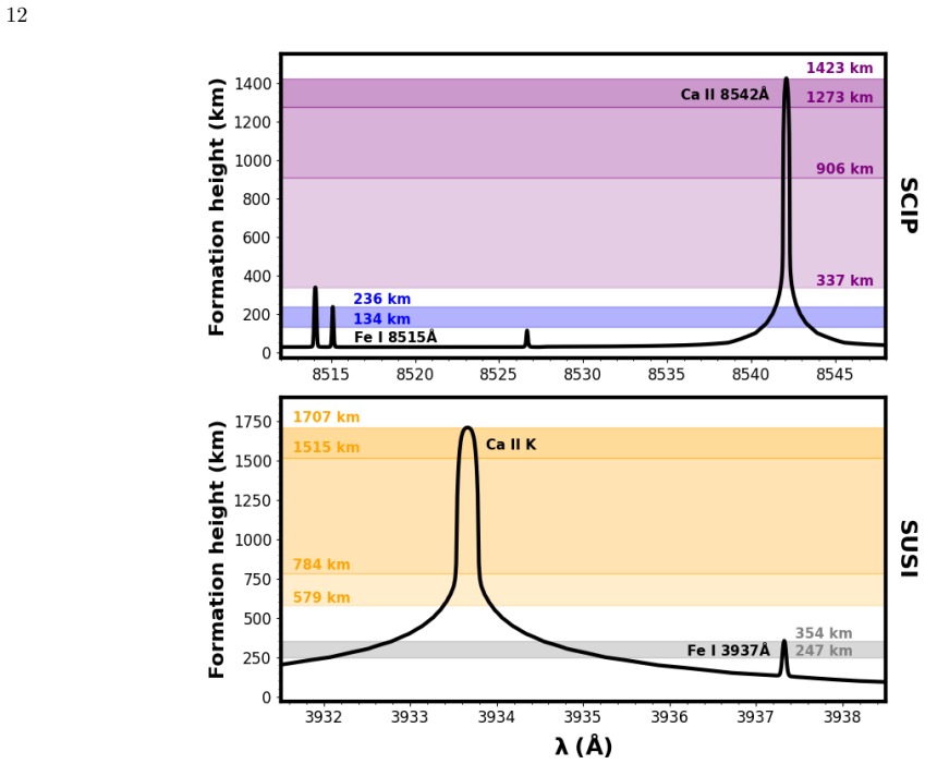
- [Appendix B; Appendix D; §4 Conclusions] Appendix B (Fig. 5) and §3–4: WFA is applied over the full Ca II lobe ranges, so each B_LOS is a formation-weighted average spanning hundreds of km. Outer-lobe τ=1 heights already overlap (Ca II K outer ~780 km vs Ca II 8542 ~900–1420 km), and Appendix D states that inner-lobe-only maps are S/N-limited over most of the FOV. The narrative that Ca II K cleanly samples ‘higher’ layers than 8542, and that the field ‘continues to expand at heights above those probed by Ca II 8542’, therefore overstates the height discrimination actually achieved. The conclusions and abstract should be rephrased to match the averaged, overlapping formation ranges, or a limited high-S/N inner-lobe subset should be shown.
- [§2 Observational data and methods] §2: SUSI and SCIP scans are separated by ~1 h and are only co-aligned via Ca II core-intensity cross-correlation. Small-scale differences between Fe I 8515 and 3937 maps are partly attributed to evolution, yet the expansion factors mix the two instruments. A quantitative bound—e.g. comparing SCIP continuum/Ca II structure at the start vs end of the SUSI window, or restricting the factor to within-instrument pairs only—would show that temporal evolution does not dominate the reported photosphere-to-chromosphere change.
minor comments (6)
- [Figure 2] Fig. 2 caption and §3: green contours are said to enclose the same magnetic flux in Ca II as in Fe I, but the text later describes a region-growing algorithm to match flux. Clarify in the caption that Ca II contours are flux-matched, not B_LOS>800 G.
- [§3 Results and discussion] §3: ‘3973 Å’ appears once where Fe I 3937 Å is meant.
- [Appendix A; Appendix C] Table 1 / Appendix A: wavelength windows for WFA/COG are given, but it is unclear whether the same windows enter the MCMC noise estimate and the COG I_wings average; a one-sentence clarification would help reproducibility.
- [Figure 1; §2] Fig. 1: continuum for SUSI is taken at 3946 Å ‘still within the wings of Ca II K’; state the expected continuum deficit or cite a quiet-Sun reference so readers can judge the I/Ic normalization.
- [Abstract; §4] Abstract and §4: ‘upper chromosphere’ for full-range Ca II K WFA is slightly strong given Appendix B heights (~1500–1700 km only for core/inner lobes). Prefer ‘middle-to-upper chromosphere’ unless inner-lobe maps are added.
- [References] References: several Sunrise III instrument papers are cited as arXiv/in press with 2025–2026 dates; ensure final bibliographic details are updated at proof.
Circularity Check
No significant circularity: observational B_LOS maps and expansion factors are computed from new Sunrise III Stokes data with standard external methods.
full rationale
The paper’s central claim—that AR-plage B_LOS weakens and the magnetized area expands by a factor of ~2 from photospheric Fe I to chromospheric Ca II—is an empirical inference from co-spatial SUSI/SCIP Stokes I,V rasters. B_LOS is obtained by applying the weak-field approximation (Landi Degl’Innocenti & Landolfi 2004) to Ca II and the center-of-gravity method (Rees & Semel 1979) to Fe I; both are textbook external techniques, not fitted to the target expansion result. Magnetized-area fractions and same-flux region-growing factors are computed directly from the resulting maps with a disclosed 20%-of-max cutoff (analogous to, but not forced by, Ishikawa et al. 2025). Self-citations (Juanikorena Berasategi et al. 2025; Kriginsky et al. 2026; instrument/CLASP papers) supply line-formation context and WFA applicability checks; they do not define or statistically force the measured B_LOS values or the factor-~2 expansion. Formation-height ordering uses an external semi-empirical model (FAL-P) as an indicative guide only. There is no self-definitional loop, no fitted parameter renamed as prediction, no load-bearing uniqueness theorem from the authors, and no renaming of a prior empirical pattern as a new derivation. The derivation chain is self-contained against the new data.
Assumptions & free parameters
free parameters (5)
- Magnetized-pixel cutoff fraction =
20% of max |B_LOS| per polarity; top 2% excluded
- WFA and COG wavelength windows =
Table 1 intervals
- WFA applicability threshold g_eff Δλ_B/Δλ_D = 0.5 =
0.5
- Same-flux patch threshold B_LOS > 800 G on Fe I =
800 G
- MCMC noise σ_V from continuum =
pixel-dependent continuum σ_V
assumptions (6)
- domain assumption Weak-field approximation: V(λ) = −4.67e−13 g_eff λ0² B_LOS ∂I/∂λ with B_LOS constant over the fitted formation region (Eq. A1).
- domain assumption Center-of-gravity method recovers B_LOS for Fe I when Zeeman splitting is not weak (Eq. C7).
- domain assumption Geometric height where τ_λ=1 in FAL-P (Fontenla et al. 1993) orders the formation of Fe I 8515, Fe I 3937, Ca II 8542, and Ca II K.
- ad hoc to paper Co-alignment by cross-correlation of Ca II core intensity maps and restriction to the common FOV make SUSI and SCIP B_LOS maps comparable despite ~1 h time gap.
- domain assumption Linear polarization can be ignored near disk center without biasing the LOS analysis.
- standard math Standard atomic/spectroscopic constants (g_eff, λ0) and the Landi Degl’Innocenti & Landolfi polarization framework.
Cite this review
Pith. "Pith review of Magnetic Field Stratification in Active-Region Plage from Ca II K and Ca II 8542 {\AA} Spectropolarimetry." pith.science (2026). https://pith.science/paper/FJZOBJKW
@misc{pith2026260728102,
  author       = {Pith},
  title        = {Pith review of: Magnetic Field Stratification in Active-Region Plage from Ca II K and Ca II 8542 \AA Spectropolarimetry},
  year         = {2026},
  howpublished = {\url{https://pith.science/paper/FJZOBJKW}},
  note         = {Machine review of arXiv:2607.28102}
}
abstract
We investigate the height variation of the line-of-sight (LOS) magnetic field in solar active-region (AR) plage from the upper photosphere to the upper chromosphere using co-spatial ultraviolet (UV) and infrared (IR) spectropolarimetric observations from the Sunrise III stratospheric balloon flight. The Ca II K and Ca II 8542 {\AA} lines provide complementary chromospheric diagnostics, while nearby Fe I lines sample photospheric layers. The LOS magnetic field is inferred from the intensity and circular polarization profiles, applying the weak field approximation for the Ca II lines and the center-of-gravity method for the Fe I lines. The photospheric Fe I lines reveal strong, finely structured magnetic fields of the order of a kG. In contrast, the chromospheric Ca II diagnostics yield systematically weaker fields, typically in the $\sim$ 100-400 G range, with a more diffuse spatial distribution. Magnetic field maps inferred from the Ca II K line, formed higher in the chromosphere, are smoother and more extended than those derived from the Ca II 8542 {\AA} line, which samples lower heights. We find that the magnetized area increases by a factor of $\sim$ 2 from the photosphere to the chromosphere. These results provide direct quantitative evidence that magnetic fields in AR plage weaken and expand with height, evolving from compact kG photospheric concentrations into weaker and more spatially extended structures in the upper chromosphere.
Figures


Figures from the paper (4 more)



Reference graph
Works this paper leans on
-
[1]
Afonso Delgado, D., del Pino Alem´ an, T., & Trujillo Bueno, J. 2023, ApJ, 954, 218, doi: 10.3847/1538-4357/ace4c8 Afonso Delgado, D., del Pino Alem´ an, T., Trujillo Bueno, J., et al. 2025, ApJ, 991, 164, doi: 10.3847/1538-4357/adfcd4 16
-
[2]
Barthol, P., Gandorfer, A., Solanki, S. K., et al. 2011, SoPh, 268, 1, doi: 10.1007/s11207-010-9662-9 Bjørgen, J. P., Sukhorukov, A. V., Leenaarts, J., et al. 2018, A&A, 611, A62, doi: 10.1051/0004-6361/201731926
-
[3]
Buehler, D., Lagg, A., Solanki, S. K., & van Noort, M. 2015, A&A, 576, A27, doi: 10.1051/0004-6361/201424970
-
[4]
2018, ApJ, 866, 89, doi: 10.3847/1538-4357/aae087 da Silva Santos, J
Centeno, R. 2018, ApJ, 866, 89, doi: 10.3847/1538-4357/aae087 da Silva Santos, J. M., Reardon, K., Cauzzi, G., et al. 2023, ApJL, 954, L35, doi: 10.3847/2041-8213/acf21f de la Cruz Rodr ´ ıguez, J., Leenaarts, J., Danilovic, S., &
-
[5]
Uitenbroek, H. 2019, A&A, 623, A74, doi: 10.1051/0004-6361/201834464 del Pino Alem´ an, T., Casini, R., & Manso Sainz, R. 2016, ApJL, 830, L24, doi: 10.3847/2041-8205/830/2/L24 del Pino Alem´ an, T., Trujillo Bueno, J., Casini, R., & Manso Sainz, R. 2020, ApJ, 891, 91, doi: 10.3847/1538-4357/ab6bc9
-
[6]
Feller, A., Gandorfer, A., Grauf, B., et al. 2025, The Sunrise Ultraviolet Spectropolarimeter and Imager: Instrument description, https://arxiv.org/abs/2504.05416
arXiv 2025
-
[7]
Fontenla, J. M., Avrett, E. H., & Loeser, R. 1993, ApJ, 406, 319, doi: 10.1086/172443
doi:10.1086/172443 1993
-
[8]
Foreman-Mackey, D., Hogg, D. W., Lang, D., & Goodman, J. 2013, PASP, 125, 306, doi: 10.1086/670067
doi:10.1086/670067 2013
Show all 27 references
-
[9]
A., Feller, A., Gandorfer, A., et al
Iglesias, F. A., Feller, A., Gandorfer, A., et al. 2025, SoPh, 300, 58, doi: 10.1007/s11207-025-02470-8
2025 doi
-
[10]
2021, Science Advances, 7, eabe8406, doi: 10.1126/sciadv.abe8406
Ishikawa, R., Trujillo Bueno, J., del Pino Alem´ an, T., et al. 2021, Science Advances, 7, eabe8406, doi: 10.1126/sciadv.abe8406
2021 doi
-
[11]
E., et al
Ishikawa, R., Trujillo Bueno, J., McKenzie, D. E., et al. 2025, ApJ, 990, 200, doi: 10.3847/1538-4357/aded0e Juanikorena Berasategi, I., Alsina Ballester, E., del Pino Alem´ an, T., & Trujillo Bueno, J. 2025, A&A, 704, A173, doi: 10.1051/0004-6361/202556353
2025 doi
-
[12]
2024, ApJ, 960, 129, doi: 10.3847/1538-4357/ad0780
Judge, P., Kleint, L., Casini, R., et al. 2024, ApJ, 960, 129, doi: 10.3847/1538-4357/ad0780
2024 doi
-
[13]
C., Solanki, S
Katsukawa, Y., del Toro Iniesta, J. C., Solanki, S. K., et al. 2026, The Sunrise Chromospheric Infrared Spectro-Polarimeter SCIP: an instrument for SUNRISE III, https://arxiv.org/abs/2603.17929
2026 arXiv
-
[14]
K., et al
Korpi-Lagg, A., Gandorfer, A., Solanki, S. K., et al. 2025, Solar Physics, 300, doi: 10.1007/s11207-025-02485-1
2025 doi
-
[15]
2026, A&A, 708, A282, doi: 10.1051/0004-6361/202558065 Landi Degl’Innocenti, E., & Landolfi, M
Danilovic, S., & Andriienko, O. 2026, A&A, 708, A282, doi: 10.1051/0004-6361/202558065 Landi Degl’Innocenti, E., & Landolfi, M. 2004, Polarization in Spectral Lines, Vol. 307, doi: 10.1007/978-1-4020-2415-3
2026 doi
-
[16]
2024a, ApJ, 975, 110, doi: 10.3847/1538-4357/ad7954
Li, H., del Pino Alem´ an, T., & Trujillo Bueno, J. 2024a, ApJ, 975, 110, doi: 10.3847/1538-4357/ad7954
-
[17]
2022, ApJ, 933, 145, doi: 10.3847/1538-4357/ac745c
Li, H., del Pino Alem´ an, T., Trujillo Bueno, J., & Casini, R. 2022, ApJ, 933, 145, doi: 10.3847/1538-4357/ac745c
2022 doi
-
[18]
2024b, ApJ, 974, 154, doi: 10.3847/1538-4357/ad6dfb Manso Sainz, R., & Trujillo Bueno, J
Li, H., del Pino Alem´ an, T., Trujillo Bueno, J., et al. 2024b, ApJ, 974, 154, doi: 10.3847/1538-4357/ad6dfb Manso Sainz, R., & Trujillo Bueno, J. 2010, ApJ, 722, 1416, doi: 10.1088/0004-637X/722/2/1416 Manso Sainz, R., & Trujillo Bueno, J. 2011, ApJ, 737, 106, doi: 10.1088/0...
2010 doi
-
[19]
2026, arXiv e-prints, arXiv:2606.16088, doi: 10.48550/arXiv.2606.16088
Matsumoto, T., Katsukawa, Y., Kubo, M., et al. 2026, arXiv e-prints, arXiv:2606.16088, doi: 10.48550/arXiv.2606.16088
2026 doi
-
[20]
2020, A&A, 642, A210, doi: 10.1051/0004-6361/202038754
Yadav, R. 2020, A&A, 642, A210, doi: 10.1051/0004-6361/202038754
2020 doi
-
[21]
Pietrow, A. G. M., Kiselman, D., de la Cruz Rodr ´ ıguez, J., et al. 2020, A&A, 644, A43, doi: 10.1051/0004-6361/202038750 Quintero Noda, C., Shimizu, T., de la Cruz Rodr ´ ıguez, J., et al. 2016, MNRAS, 459, 3363, doi: 10.1093/mnras/stw867
2020 doi
-
[22]
E., & Semel, M
Rees, D. E., & Semel, M. D. 1979, A&A, 74, 1
1979
-
[23]
2000, Science, 288, 1396, doi: 10.1126/science.288.5470.1396
Socas-Navarro, H., Trujillo Bueno, J., & Ruiz Cobo, B. 2000, Science, 288, 1396, doi: 10.1126/science.288.5470.1396
2000
-
[24]
K., Barthol, P., Danilovic, S., et al
Solanki, S. K., Barthol, P., Danilovic, S., et al. 2010, ApJL, 723, L127, doi: 10.1088/2041-8205/723/2/L127
2010 doi
-
[25]
K., Riethm¨ uller, T
Solanki, S. K., Riethm¨ uller, T. L., Barthol, P., et al. 2017, ApJS, 229, 2, doi: 10.3847/1538-4365/229/1/2
2017 doi
- [26]
-
[27]
Vissers, G. J. M., Danilovic, S., Zhu, X., et al. 2022, A&A, 662, A88, doi: 10.1051/0004-6361/202142087
2022 doi
Reviewed July 31, 2026 · model on record in the stance chip above.
Discussion (0). Sign in to comment.