REVIEW 3 major objections 6 minor 29 references
Bring the Heat: Rapid Trajectory Optimization with Pseudospectral Techniques and the Affine Geometric Heat Flow Equation
T0 review · 3 major / 6 minor · reviewed 2026-08-12 · deepseek-v4-flash
Pith's one-line read The paper claims PHLAME can plan a 44-dimensional pinned humanoid trajectory in about five seconds by solving the Affine Geometric Heat Flow PDE with pseudospectral collocation and spatial-vector rigid-body dynamics.
desk verdict Fast and useful for fully actuated systems, but the analytical AGHF is only proven for B=I, not the general case claimed. read the letter →
The pith
A machine-rendered reading of the paper's core claim, the machinery that carries it, and where it could break.
The reading
What carries the argument
The load-bearing object is the Affine Geometric Heat Flow PDE, defined by $$\frac{\partial x}{\partial s}=$G^{{-1}}$(x)\left(\frac{d}{dt}\frac{\partial L}{\partial \dot x}-\frac{\partial L}{\partial x}\right),$$ with boundary conditions $x_s(0)=x_0$ and $x_s(T)=x_f$. The identity that carries the computation is the choice $G=(\bar F^{-1})^T K \bar F^{-1}$, which makes the action functional equal $\int_0^T (k\|\dot x_{P1}-x_{P2}\|^2+\|u_s\|^2)\,dt$; Theorem 5 rewrites the right-hand side as $\Omega_1-(\Omega_2-\Omega_3+\Omega_4)$, with each $\Omega_i$ a combination of rigid-body quantities such as $H$, $C$, $\dot H$, $\dot C$, and $F_{D0}$ that recursive spatial-vector algorithms evaluate without forming large symbolic expressions. The second mechanism is the Chebyshev pseudospectral method of lines: replacing time derivatives with a differentiation matrix $D$ turns the PDE into the ODE system $d\xi/ds=\Omega(\xi,D\xi,D^2\xi,k)$ on the Chebyshev nodes, so a handful of nodes yields high-accuracy derivatives. The third is Theorem 6's analytical Jacobian of that ODE right-hand side, which lets an implicit ODE solver avoid finite-difference derivative approximations.
What would settle it
Evaluate the AGHF right-hand side for a simple underactuated system, such as a two-link pendulum driven by a single motor so that B is non-identity, using both a numerical differentiation of the original definition (7) and the closed form in Theorem 5; if the two differ at generic states, the closed form is not the AGHF of the stated dynamics, and PHLAME's reported speed applies to a different problem.
Extended reading notes
Core claim
On the paper's own terms, the central discovery is that the AGHF PDE, whose solution domain is two-dimensional regardless of state dimension, can be solved for real robots by combining three ingredients: Chebyshev pseudospectral collocation in time; an analytical form of the AGHF right-hand side (Theorem 5) expressed solely through the mass matrix, the Coriolis and gravity term, their derivatives, and forward-dynamics quantities; and an analytical Jacobian (Theorem 6) that lets an implicit ODE solver avoid finite-difference derivative estimates. The paper reports that PHLAME evaluates the AGHF right-hand side in about 105 microseconds for the 22-body pinned Digit, solves a 7-DOF arm trajectory in about 0.2 to 0.3 seconds, and solves pinned Digit stepping and stretching problems in about 3.3 to 5.3 seconds, with success under the paper's forward-simulation criterion. The same pipeline succeeds with obstacle constraints on both the arm and the humanoid, while the original AGHF implementation could not even generate the symbolic right-hand side beyond five bodies.
Load-bearing premise
The load-bearing premise is that in the derivation of the closed-form AGHF it is harmless to assume the actuation matrix B (the matrix mapping motor commands to joint forces) is the identity; if that assumption is not actually without loss of generality, then for underactuated or differently actuated robots PHLAME solves a different PDE from the one whose convergence theory justifies the method.
Editorial extensions
If this is right
- A 44-dimensional state-space system (pinned Digit V3) can be optimized in about three to five seconds, including obstacle cases, under PHLAME's success criterion.
- The AGHF right-hand side evaluation is roughly 10 to 1000 times faster than the original AGHF implementation; beyond five bodies the original symbolic implementation did not finish, whereas PHLAME scales to 22 bodies.
- Obstacle avoidance can be folded into the PDE through a smooth penalty in the Lagrangian, and PHLAME completed all Digit stepping trials with obstacle radii up to 20.3 centimeters within the success threshold.
- Because the Jacobian is supplied analytically, implicit ODE integration avoids finite-difference derivative evaluations, further cutting the number of function evaluations required.
- The penalty-based incorporation of constraints means PHLAME's trajectories are dynamically feasible to within the penalty tolerance, not necessarily the exact control-minimizing solutions of the original constrained optimal control problem.
Reading between the lines
- A direct extension the authors do not work out is to use PHLAME's seconds-fast solution as a warm start for a local optimal-control refinement; this would directly address the paper's own admission that the penalty formulation does not fully minimize control effort.
- The reported scaling fits, in which AGHF evaluation time grows roughly quadratically in body count over 2 to 22 bodies, suggest the method could reach still larger humanoids, but only after the identity-actuation assumption is removed for underactuated systems.
- Because pseudospectral accuracy depends on solution smoothness, PHLAME's obstacle performance could degrade if the constraint activation function is made very sharp; a steeper tanh penalty trades differentiability for constraint sharpness.
- The same pseudospectral method-of-lines treatment could apply to other PDE-based motion planners whose solution domains are low-dimensional, transferring the speedup beyond the AGHF setting.
Editorial analysis
A structured set of objections, weighed in public.
Referee Report
Summary. The paper presents PHLAME, a trajectory-optimization method that solves the Affine Geometric Heat Flow (AGHF) PDE by pseudospectral collocation in time and by evaluating the AGHF and its Jacobian through spatial-vector-algebra rigid-body-dynamics algorithms. The authors derive closed-form expressions for the AGHF right-hand side (Theorem 5) and its Jacobian (Theorem 6) for a fully actuated version of the dynamics in (1), describe Algorithms 2 and 3 for evaluating these quantities, and report experiments on pendulum chains, the Kinova Gen3 arm, and a modified pinned Digit model, with and without obstacle constraints. The headline empirical result is solving a 44-dimensional state-space Digit model in about 5 seconds, substantially faster than the reported Crocoddyl and Aligator baselines.
Significance. If the technical gaps are repaired, the paper would make a credible contribution: it turns a PDE-based motion-planning method that previously could not scale beyond a handful of bodies into one that handles a 22-DOF (44-state) humanoid-scale model in seconds. The use of analytical derivatives and spatial-vector algorithms is a principled way to reduce per-evaluation cost, and the paper provides parameter tables and a project page that aid reproducibility. The speed comparisons with DDP baselines, while not a formal complexity guarantee, are informative. The main reservations are analytical: the derivation of the closed-form AGHF is only valid for B=I and m=N, and the smooth constraint penalty in Section V is not exactly the stated one, so the currently stated generality of the method exceeds what is proven.
major comments (3)
- [Appendix A, Eqs. (35)–(36)] The step 'we assume, without loss of generality (WLOG), that B = I' is not valid for general actuation matrices. Replacing B by I changes the cost in (OCP) unless B is a scalar multiple of an orthogonal matrix, because the same physical control effort ∥u∥² is not preserved under u' = Bu. For B ≠ I, the lower-right block of G in Lemma 4 is H^T B^{-T} B^{-1} H, and Ω2–Ω4 in Eqs. (17)–(19) depend on B through \bar F^{-1}; none of the formulas in Theorem 5 contains B. Moreover, the displayed block form of \bar F^{-1} in Eq. (35) requires B to be square, so the derivation also assumes m=N. Because Theorem 5 and Theorem 6 feed directly into Algorithm 2, Algorithm 3, and Algorithm 1, PHLAME as presented is only guaranteed to solve the stated OCP when B=I and the system is fully actuated. The experiments appear to satisfy this restriction, so the empirical speed claims are not invalidated, but the paper's stated generality to all systems of form (1) is unsupported; either the general-B derivation should be supplied or the claims and theorems should be restricted accordingly.
- [Section V-A, Definition 7 and Eq. (30)] The defining conditions on S are mutually inconsistent with differentiability: a differentiable function cannot be identically 0 on g≤0 and identically 1 on g>0 because that would require a jump at g=0. The proposed example in Eq. (30) is strictly between 0 and 1 for every nonzero g and therefore violates both conditions. As a result, the penalty b(g_j) in Eq. (29) does not vanish for feasible configurations and under-penalizes violated configurations, so the constrained AGHF in Definition 8 minimizes a different functional from the one claimed. Since the obstacle experiments all use the tanh switch in Eq. (30), this is a gap in the constrained part of the method; the paper should replace Definition 7 with a precise smooth-surrogate formulation or prove convergence for the actual S used.
- [Section V, Definition 8] The convergence of the constrained AGHF is asserted by reference to [28, Lemma 4.1], but the lemma's hypotheses are not stated and no verification is given that the multi-constraint penalty (28) with the smooth switch (30) satisfies them. Given that obstacle avoidance is a headline result (Tables IV–VI), the paper should either state and verify the assumptions or provide a self-contained convergence argument; otherwise the constrained claims rest on an imported theorem whose applicability is not established.
minor comments (6)
- [Section IV-B, Eqs. (22)–(23)] The notation for dξ_i/ds is dimensionally inconsistent because ξ_i(s) is a row vector in Eq. (21) while Ω takes a column vector; the paper's 'abuse of notation' should be replaced by an explicit convention, such as defining all quantities as columns, so that Eqs. (22)–(23) are unambiguous.
- [Algorithm 1 and Section VI-A3] The integration in s is not reproducible as described: the paper never names the ODE solver or gives its tolerances, despite stating that an implicit method is used; please report the solver and settings used for the timings.
- [Section IV-A] The sentence introducing Algorithm 2 says it 'computes the expressions introduced in Algorithm 2'; it should refer to Theorem 5.
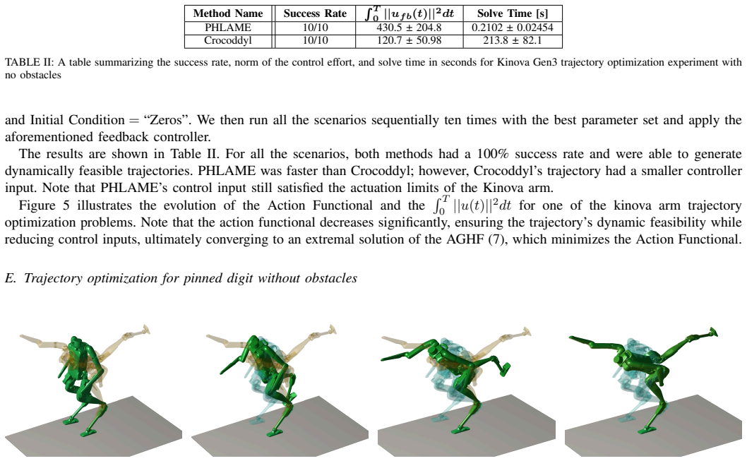
- [Section VI-D–G] In the comparison tables, PHLAME's reported ∫||u_fb||² values are consistently larger than those of Crocoddyl or Aligator; the paper should state explicitly that the speed advantage is obtained at the cost of higher control effort, since the baselines optimize an augmented cost that includes state and terminal terms.
- [Section VI-A1] The paper should consistently describe the Digit experiments as using a modified, fully actuated model with the closed kinematic chains removed, and qualify the '44-dimensional state-space system' claim accordingly, since this is not the stock Digit V3 platform.
- [Section VII] The conclusion's claim of being 'much faster than state-of-the-art trajectory optimization methods' should be qualified to the compared methods (Crocoddyl, Aligator, and the original AGHF), since direct collocation methods such as C-FROST, TROPIC, and RAPTOR are not benchmarked.
Circularity Check
No significant circularity: the analytical AGHF and Jacobian are direct algebraic expansions, and all benchmark claims are evaluated against external solvers.
full rationale
The paper's central derivation is Theorem 5, whose proof in Appendix A substitutes the G from Lemma 4 into the AGHF PDE from Definition 2 and expands the Euler-Lagrange expression; this is a self-contained algebraic derivation, not a fitted parameter renamed as a prediction. Lemma 4 and the convergence guarantees are attributed to [16] and [28], external works by different authors, and the pseudospectral transcription in Section IV-B uses standard Chebyshev differentiation matrices and standard convergence theory. The empirical speed claims are benchmarked against Crocoddyl, Aligator, and the original AGHF implementation, all external to the present paper. Hyperparameters are grid-searched and disclosed, and no reported output is forced by construction. The only load-bearing weakness, the 'WLOG B=I' step in Appendix A Eqs. (35)-(36), is an invalid generality assumption for non-identity actuation matrices; this is a correctness gap, not a circularity. Since no prediction reduces to an input by definition and no load-bearing self-citation exists, the paper deserves a 0 on the circularity scale.
Assumptions & free parameters
free parameters (5)
- k =
1e3 to 1e10 per experiment via grid search
- smax =
1e-4 to 100 per experiment via grid search
- p =
5 to 15 per experiment via grid search
- kcons =
1e5 to 1e10 for obstacle experiments
- ccons =
1 to 200 for obstacle experiments
assumptions (6)
- domain assumption Assumption 1: Fd and F are C^2, Lipschitz continuous, F has constant rank almost everywhere, and a feasible solution to the motion planning problem exists.
- domain assumption The AGHF PDE converges to a trajectory that is arbitrarily close to feasible for sufficiently large k and smax ([16, Theorem 1]).
- domain assumption The constrained AGHF with penalty term b(g_j) converges to a solution satisfying the constraints ([28, Lemma 4.1]).
- standard math The pseudospectral method of lines converges to the true PDE solution under certain regularity conditions ([20, Ch. 9 and 12]).
- standard math The completion Fc in Lemma 4 exists and makes [Fc, F] invertible (via Gram-Schmidt).
- ad hoc to paper B can be set to the identity matrix without loss of generality.
Cite this review
Pith. "Pith review of Bring the Heat: Rapid Trajectory Optimization with Pseudospectral Techniques and the Affine Geometric Heat Flow Equation." pith.science (2026). https://pith.science/paper/FO5DEU2V
@misc{pith2026241112962,
  author       = {Pith},
  title        = {Pith review of: Bring the Heat: Rapid Trajectory Optimization with Pseudospectral Techniques and the Affine Geometric Heat Flow Equation},
  year         = {2026},
  howpublished = {\url{https://pith.science/paper/FO5DEU2V}},
  note         = {Machine review of arXiv:2411.12962}
}
abstract
Generating optimal trajectories for high-dimensional robotic systems in a time-efficient manner while adhering to constraints is a challenging task. This paper introduces PHLAME, which applies pseudospectral collocation and spatial vector algebra to efficiently solve the Affine Geometric Heat Flow (AGHF) Partial Differential Equation (PDE) for trajectory optimization. Unlike traditional PDE approaches like the Hamilton-Jacobi-Bellman (HJB) PDE, which solve for a function over the entire state space, computing a solution to the AGHF PDE scales more efficiently because its solution is defined over a two-dimensional domain, thereby avoiding the intractability of state-space scaling. To solve the AGHF one usually applies the Method of Lines (MOL), which discretizes one variable of the AGHF PDE, and converts the PDE into a system of ordinary differential equations (ODEs) that are solved using standard time-integration methods. Though powerful, this method requires a fine discretization to generate accurate solutions and requires evaluating the AGHF PDE which is computationally expensive for high-dimensional systems. PHLAME overcomes this deficiency by using a pseudospectral method, which reduces the number of function evaluations required to yield a high accuracy solution thereby allowing it to scale efficiently to high-dimensional robotic systems. To further increase computational speed, this paper presents analytical expressions for the AGHF and its Jacobian, both of which can be computed efficiently using rigid body dynamics algorithms. PHLAME is tested across various dynamical systems, with and without obstacles and compared to a number of state-of-the-art techniques. PHLAME generates trajectories for a 44-dimensional state-space system in $\sim5$ seconds, much faster than current state-of-the-art techniques. A project page is available at https://roahmlab.github.io/PHLAME/
Figures


Figures from the paper (5 more)




Reference graph
Works this paper leans on
-
[16]
Affine geometric heat flow and motion planning for dynamic systems,
S. Liu, Y . Fan, and M.-A. Belabbas, “Affine geometric heat flow and motion planning for dynamic systems,” IFAC-PapersOnLine, vol. 52, no. 16, pp. 168–173, 2019, 11th IFAC Symposium on Nonlinear Control Systems NOLCOS 2019
work page 2019
-
[28]
Robot motion planning via curve shortening flows,
Y . Fan, “Robot motion planning via curve shortening flows,” Ph.D. dissertation, University of Illinois at Urbana-Champaign, 2021
work page 2021
-
[1]
Agile and versatile climbing on ferromagnetic surfaces with a quadrupedal robot,
S. Hong, Y . Um, J. Park, and H.-W. Park, “Agile and versatile climbing on ferromagnetic surfaces with a quadrupedal robot,” Science Robotics, vol. 7, no. 73, eadd1017, 2022
work page 2022
-
[2]
Generating continuous motion and force plans in real-time for legged mobile manipulation,
P. Ewen, J.-P. Sleiman, Y . Chen, W.-C. Lu, M. Hutter, and R. Vasudevan, “Generating continuous motion and force plans in real-time for legged mobile manipulation,” in 2021 IEEE international conference on robotics and automation (ICRA) , IEEE, 2021, pp. 4933–4939
work page 2021
-
[3]
Let's Make a Splan: Risk-Aware Trajectory Optimization in a Normalized Gaussian Splat
J. Michaux, S. Isaacson, C. E. Adu, et al. , “Let’s make a splan: Risk-aware trajectory optimization in a normalized gaussian splat,” arXiv preprint arXiv:2409.16915 , 2024
work page Pith review arXiv 2024
-
[4]
Dynamic locomotion in the mit cheetah 3 through convex model-predictive control,
J. Di Carlo, P. M. Wensing, B. Katz, G. Bledt, and S. Kim, “Dynamic locomotion in the mit cheetah 3 through convex model-predictive control,” in 2018 IEEE/RSJ International Conference on Intelligent Robots and Systems (IROS) , 2018, pp. 1–9
work page 2018
-
[5]
J. Liu, C. E. Adu, L. Lymburner, V . Kaushik, L. Trang, and R. Vasudevan, Radius: Risk-aware, real-time, reachability-based motion planning, 2023
work page 2023
-
[6]
Mini cheetah: A platform for pushing the limits of dynamic quadruped control,
B. Katz, J. D. Carlo, and S. Kim, “Mini cheetah: A platform for pushing the limits of dynamic quadruped control,” in 2019 International Conference on Robotics and Automation (ICRA) , 2019, pp. 6295–6301
work page 2019
Show all 29 references
-
[7]
Bertsekas, Dynamic programming and optimal control: Volume I
D. Bertsekas, Dynamic programming and optimal control: Volume I . Athena scientific, 2012, vol. 4
2012
-
[8]
Crocoddyl: An efficient and versatile framework for multi-contact optimal control,
C. Mastalli, R. Budhiraja, W. Merkt, et al. , “Crocoddyl: An efficient and versatile framework for multi-contact optimal control,” in 2020 IEEE International Conference on Robotics and Automation (ICRA) , 2020, pp. 2536–2542
2020
-
[9]
Jallet, A
W. Jallet, A. Bambade, E. Arlaud, S. El-Kazdadi, N. Mansard, and J. Carpentier, PROXDDP: Proximal Constrained Trajectory Optimization, https://inria.hal.science/hal-04332348v1, 2023
2023
-
[10]
Rapid trajectory optimization using c-frost with illustration on a cassie-series dynamic walking biped,
A. Hereid, O. Harib, R. Hartley, Y . Gong, and J. W. Grizzle, “Rapid trajectory optimization using c-frost with illustration on a cassie-series dynamic walking biped,” in 2019 IEEE/RSJ International Conference on Intelligent Robots and Systems (IROS) , 2019, pp. 4722–4729
2019
-
[11]
Rapid bipedal gait optimization in casadi,
M. Fevre, P. M. Wensing, and J. P. Schmiedeler, “Rapid bipedal gait optimization in casadi,” in 2020 IEEE/RSJ International Conference on Intelligent Robots and Systems (IROS) , 2020, pp. 3672–3678
2020
-
[12]
The energetic benefit of robotic gait selection—a case study on the robot ramone,
N. Smit-Anseeuw, R. Gleason, R. Vasudevan, and C. D. Remy, “The energetic benefit of robotic gait selection—a case study on the robot ramone,” IEEE Robotics and Automation Letters , vol. 2, no. 2, pp. 1124–1131, 2017
2017
-
[13]
Walking with confidence: Safety regulation for full order biped models,
N. Smit-Anseeuw, C. D. Remy, and R. Vasudevan, “Walking with confidence: Safety regulation for full order biped models,” IEEE Robotics and Automation Letters , vol. 4, no. 4, pp. 4177–4184, 2019
2019
-
[14]
Zhang and R
B. Zhang and R. Vasudevan, Rapid and robust trajectory optimization for humanoids , 2024
2024
-
[15]
The maximum principle of pontryagin in control and in optimal control,
A. D. Lewis, “The maximum principle of pontryagin in control and in optimal control,” Handouts for the course taught at the Universitat Politecnica de Catalunya, 2006
2006
-
[17]
W. E. Schiesser, The numerical method of lines: integration of partial differential equations . Elsevier, 2012
2012
-
[18]
A homotopy method for motion planning,
S. Liu and M. A. Belabbas, “A homotopy method for motion planning,” arXiv preprint arXiv:1901.10094 , 2019
1901 arXiv
-
[19]
Geometric motion planning for affine control systems with indefinite boundary conditions and free terminal time,
S. Liu, Y . Fan, and M.-A. Belabbas, “Geometric motion planning for affine control systems with indefinite boundary conditions and free terminal time,” arXiv preprint arXiv:2001.04540 , 2020
2001 arXiv
-
[20]
J. P. Boyd, Chebyshev and Fourier spectral methods . Courier Corporation, 2001
2001
-
[21]
L. N. Trefethen, Approximation Theory and Approximation Practice, Extended Edition . SIAM, 2019
2019
-
[22]
Implicit-explicit runge-kutta schemes for stiff systems of differential equations,
L. Pareschi, G. Russo, et al., “Implicit-explicit runge-kutta schemes for stiff systems of differential equations,” Recent trends in numerical analysis, vol. 3, pp. 269–289, 2000
2000
-
[23]
On second-order derivatives of rigid-body dynamics: Theory & implementation,
S. Singh, R. P. Russell, and P. M. Wensing, “On second-order derivatives of rigid-body dynamics: Theory & implementation,” IEEE Transactions on Robotics , 2024
2024
-
[24]
The pinocchio c++ library : A fast and flexible implementation of rigid body dynamics algorithms and their analytical derivatives,
J. Carpentier, G. Saurel, G. Buondonno, et al., “The pinocchio c++ library : A fast and flexible implementation of rigid body dynamics algorithms and their analytical derivatives,” in 2019 IEEE/SICE International Symposium on System Integration (SII), 2019, pp. 614–619
2019
-
[25]
Analytical Derivatives of Rigid Body Dynamics Algorithms,
J. Carpentier and N. Mansard, “Analytical Derivatives of Rigid Body Dynamics Algorithms,” in Robotics: Science and Systems (RSS 2018), Pittsburgh, United States, Jun. 2018
2018
-
[26]
Efficient analytical derivatives of rigid-body dynamics using spatial vector algebra,
S. Singh, R. P. Russell, and P. M. Wensing, “Efficient analytical derivatives of rigid-body dynamics using spatial vector algebra,” IEEE Robotics and Automation Letters , vol. 7, no. 2, 1776–1783, Apr. 2022
2022
-
[27]
Mid-air motion planning of robot using heat flow method with state constraints,
Y . Fan, S. Liu, and M.-A. Belabbas, “Mid-air motion planning of robot using heat flow method with state constraints,” Mechatronics, vol. 66, p. 102 323, 2020
2020
-
[29]
Optimization-based control for dynamic legged robots,
P. M. Wensing, M. Posa, Y . Hu, A. Escande, N. Mansard, and A. D. Prete, “Optimization-based control for dynamic legged robots,” IEEE Transactions on Robotics , vol. 40, pp. 43–63, 2024. APPENDIX A PROOF OF THEOREM 5 Proof: The Affine Geometric Heat Flow (AGHF) Equation is giv...
2024
Reviewed August 12, 2026 · model on record in the stance chip above.
Discussion (0). Continue with ORCID to comment.